| Metric | 0.02 | 0.04 | 0.06 | 0.08 | 0.10 |
|---|---|---|---|---|---|
| \(W\) corrected \(R^2\) | 0.9606 | 0.9253 | 0.8747 | 0.8138 | 0.7558 |
| \(W\) corrected slope | 0.9339 | 0.8228 | 0.6835 | 0.5830 | 0.5096 |
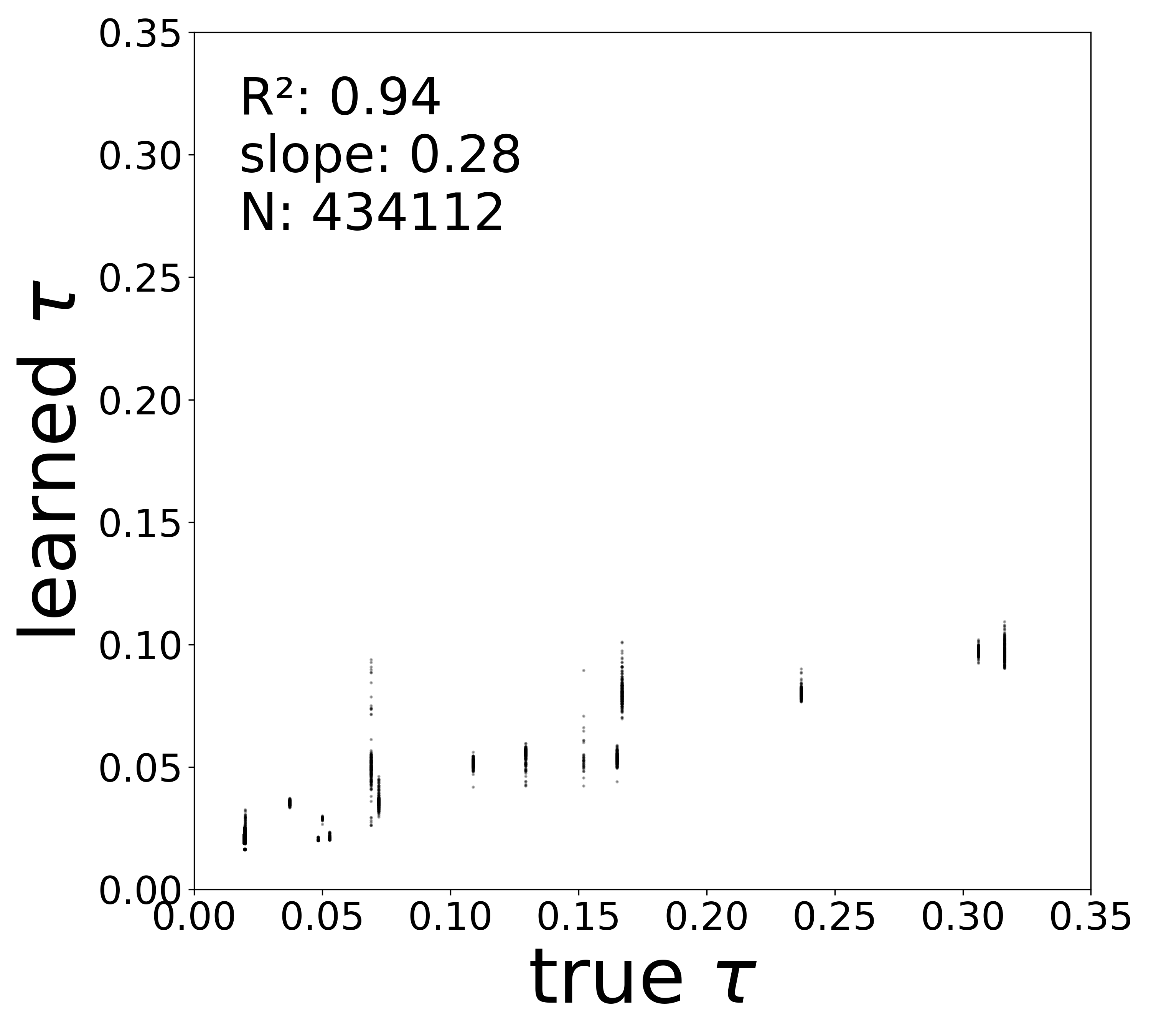
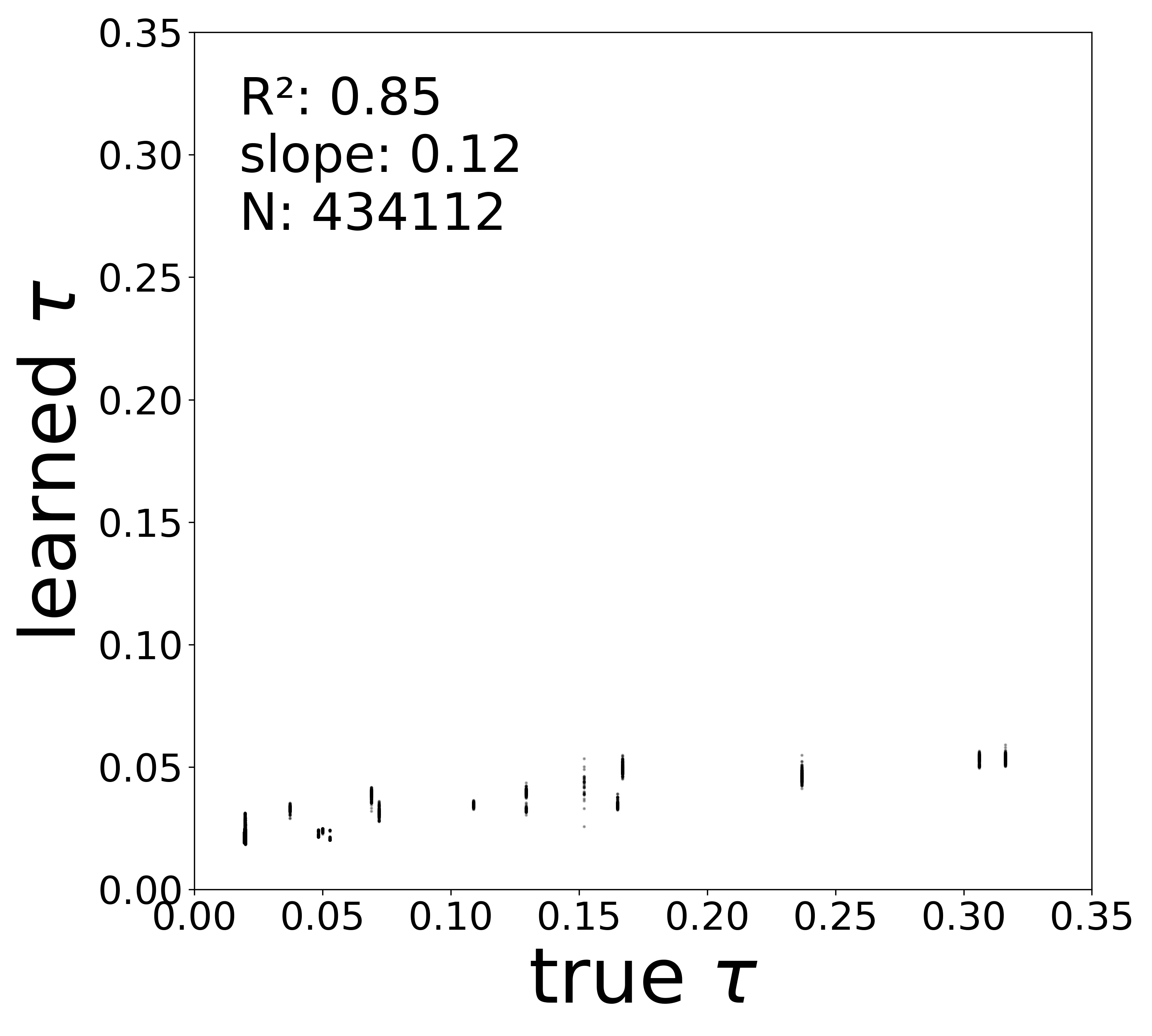
| \(\tau\) \(R^2\) | 0.9806 | 0.9674 | 0.9367 | 0.9045 | 0.8471 |
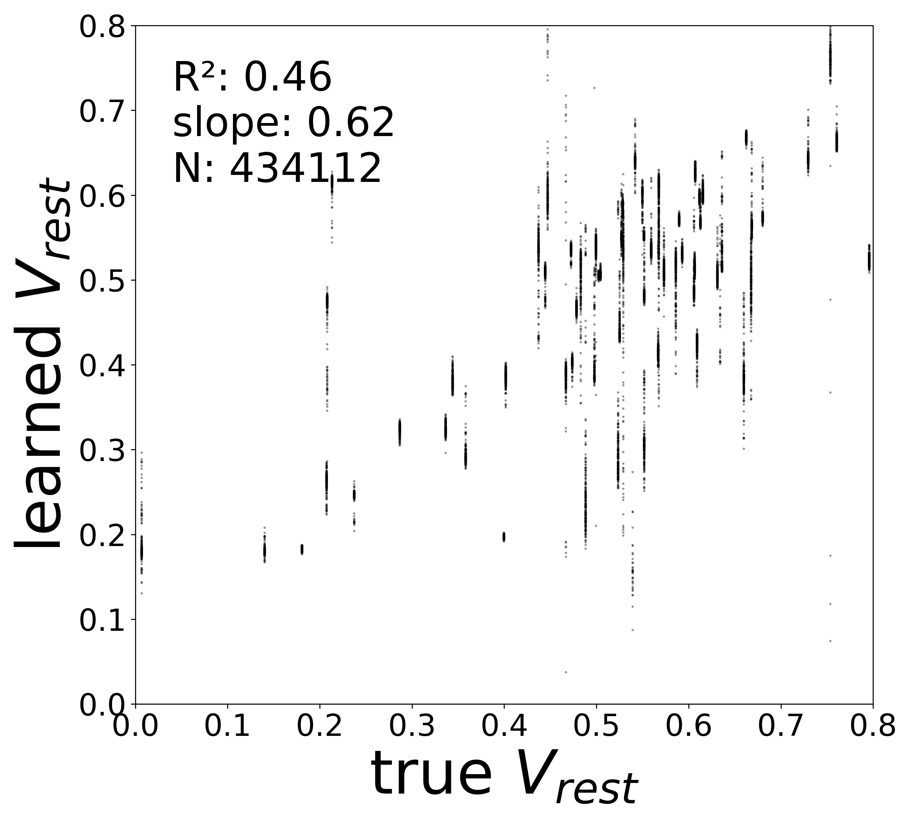
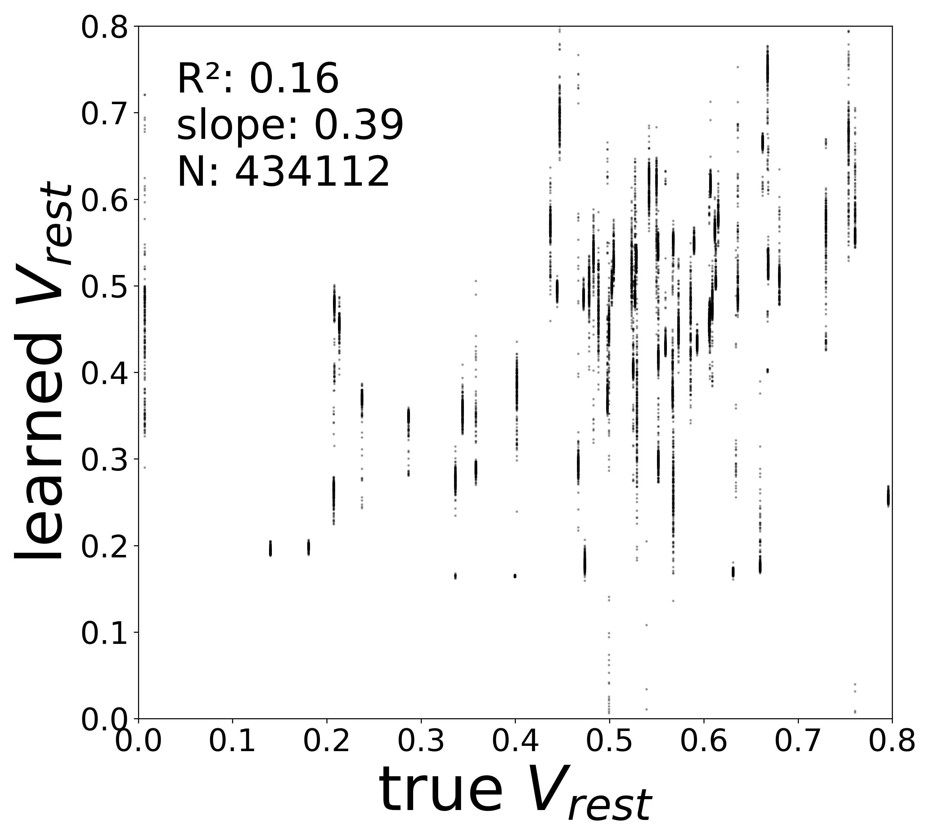
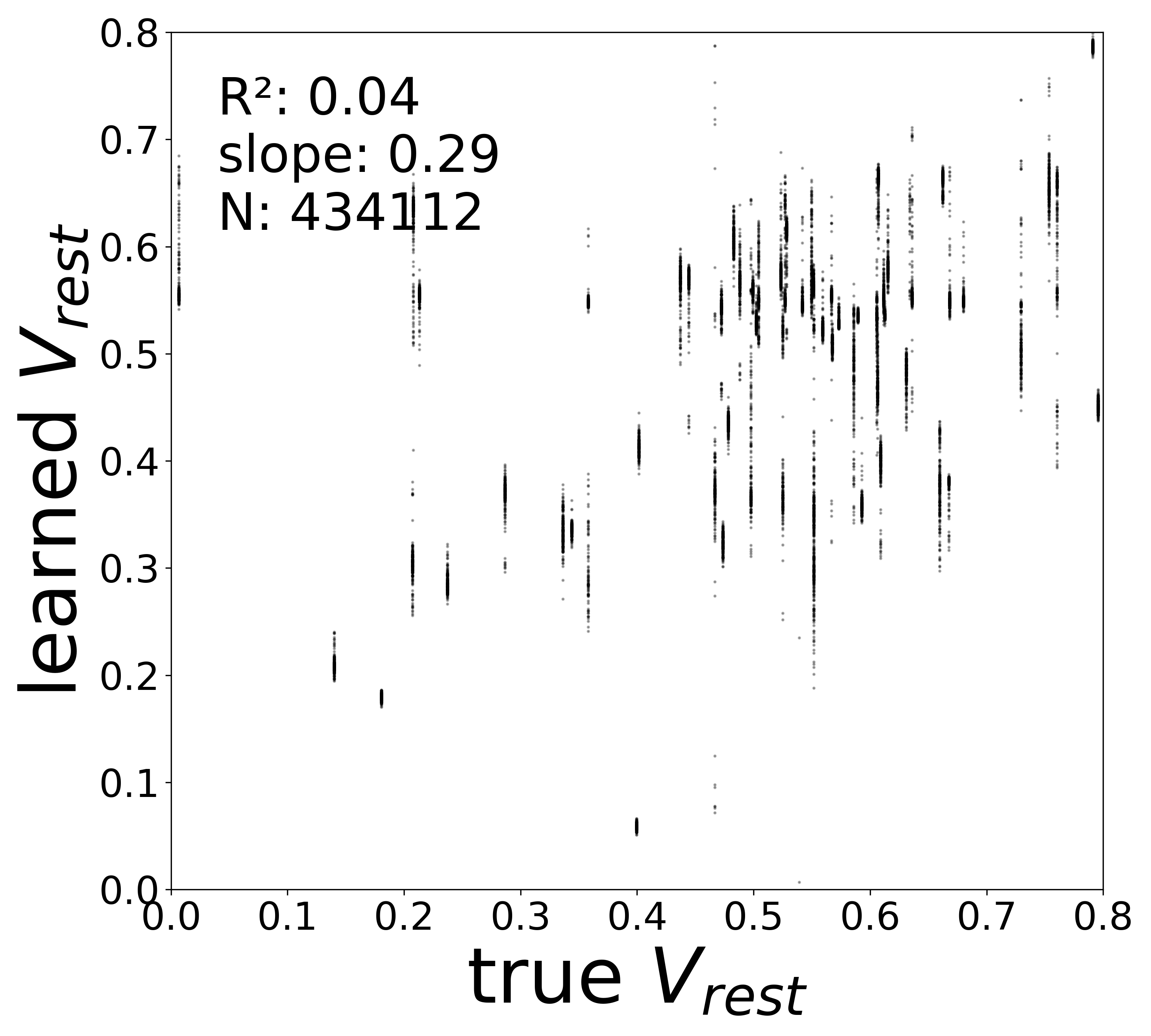
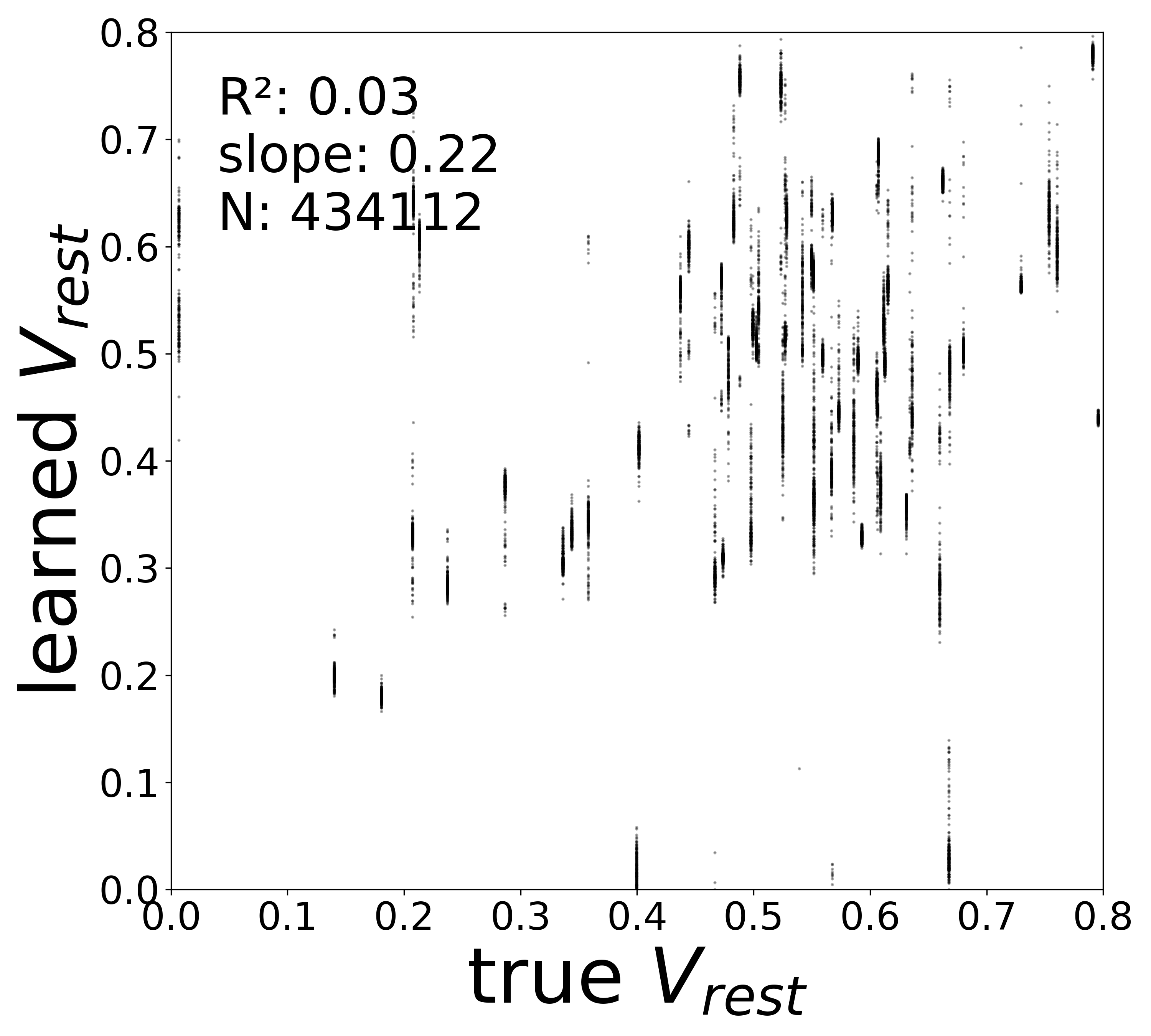
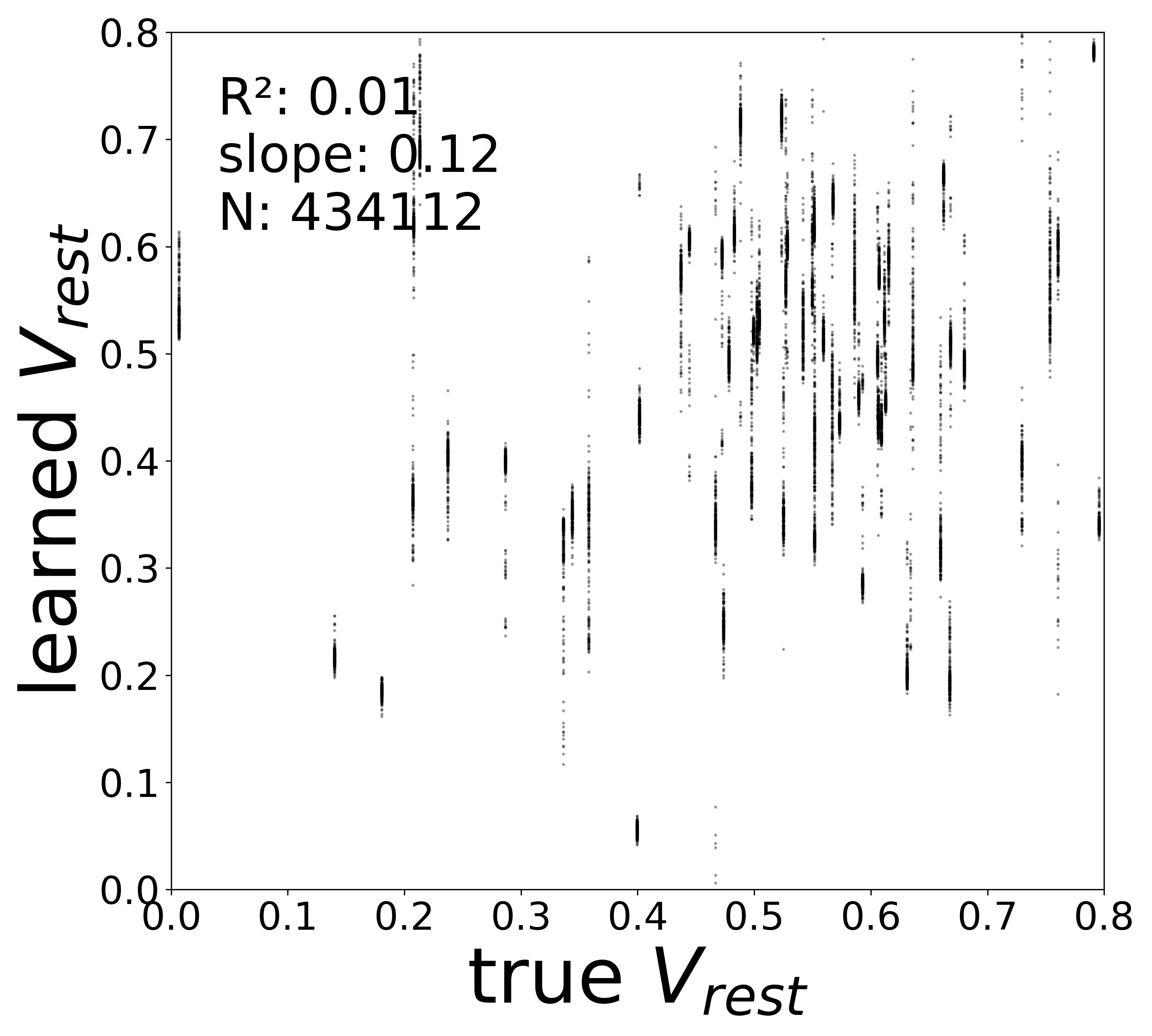
| \(V^{\text{rest}}\) \(R^2\) | 0.4563 | 0.1601 | 0.0409 | 0.0300 | 0.0079 |
Robustness to Measurement Noise
FlyVis
GNN
Measurement Noise
Train the GNN on voltage observations corrupted by additive Gaussian measurement noise at five levels. Evaluate whether the model can still recover synaptic weights, biophysical parameters, and neuron-type identity from noisy observations.
Robustness to Measurement Noise
In all previous experiments, the GNN received clean voltage traces from the simulator (up to intrinsic dynamics noise). In a real experimental setting, however, voltage recordings are corrupted by measurement noise — instrument noise, shot noise, or fluorescence noise in calcium imaging. This notebook investigates how measurement noise degrades the GNN’s ability to recover the circuit.
Distinction Between Intrinsic and Measurement Noise
Recall the simulated dynamics (Notebook 00):
\[\tau_i\frac{dv_i(t)}{dt} = -v_i(t) + V_i^{\text{rest}} + \sum_{j\in\mathcal{N}_i} \mathbf{W}_{ij}\, \text{ReLU}\!\big(v_j(t)\big) + I_i(t) + \sigma_{\text{dyn}}\,\xi_i(t),\]
where \(\sigma_{\text{dyn}}\,\xi_i(t)\) with \(\xi_i(t) \sim \mathcal{N}(0,1)\) is intrinsic dynamics noise that drives stochastic fluctuations within the ODE. This noise is part of the true dynamics and produces voltage trajectories that genuinely differ from the deterministic solution.
Measurement noise is fundamentally different: it corrupts the observations of the voltage, not the dynamics themselves. The GNN receives
\[\tilde{v}_i(t) = v_i(t) + \sigma_{\text{meas}}\,\eta_i(t), \qquad \eta_i(t) \sim \mathcal{N}(0,1),\]
and the derivative targets become
\[\frac{d\widetilde{v}}{dt} \approx \frac{\tilde{v}_i(t+\Delta t) - \tilde{v}_i(t)}{\Delta t},\]
which amplifies the measurement noise by a factor \(\sim 1/\Delta t\). Both the input voltage and the derivative targets are noisy, making this a harder inverse problem than intrinsic noise alone.
Experimental Setup
We fix the intrinsic dynamics noise at \(\sigma_{\text{dyn}} = 0.05\) (the same as the baseline Notebook 04 low-noise condition) and vary the measurement noise level across five conditions:
| Config | \(\sigma_{\text{meas}}\) | Voltage SNR | Derivative SNR |
|---|---|---|---|
flyvis_noise_005_002 |
0.02 | high | moderate |
flyvis_noise_005_004 |
0.04 | moderate | low |
flyvis_noise_005_006 |
0.06 | moderate | low |
flyvis_noise_005_008 |
0.08 | low | very low |
flyvis_noise_005_010 |
0.10 | low | very low |
To change the intrinsic noise level, edit noise_model_level in the respective config files under config/fly/.
Results
Each config shares the same intrinsic dynamics noise (\(\sigma_{\text{dyn}} = 0.05\)) and GNN architecture. Only the measurement noise level \(\sigma_{\text{meas}}\) varies.
Optimized Training Hyperparameters
A systematic LLM-driven exploration on the \(\sigma_{\text{meas}} = 0.04\) condition (36 iterations across 5 intervention categories) identified noise-robust hyperparameters that significantly improve connectivity recovery under measurement noise:
| Parameter | Default | Optimized | Rationale |
|---|---|---|---|
batch_size |
4 | 6 | Larger batches average out noisy gradients |
data_augmentation_loop |
35 | 30 | Balances noise averaging with convergence |
coeff_g_phi_diff |
750 | 1200 | Stronger monotonicity constraint stabilizes \(g_\phi\) |
These parameters are applied uniformly across all five measurement noise conditions. The exploration also established that noise averaging (batch size \(\times\) augmentation loop) is the dominant lever — all other interventions tested (LR scheduling, recurrent training, derivative smoothing, stronger L1/L2 regularization, \(f_\theta\) message monotonicity) either degraded or catastrophically broke training.
On the \(\sigma_{\text{meas}} = 0.04\) condition, the optimized config achieves connectivity \(R^2 = 0.925 \pm 0.003\) (CV = 0.3% across 4 seeds), compared to \(R^2 \approx 0.82\) with default parameters.
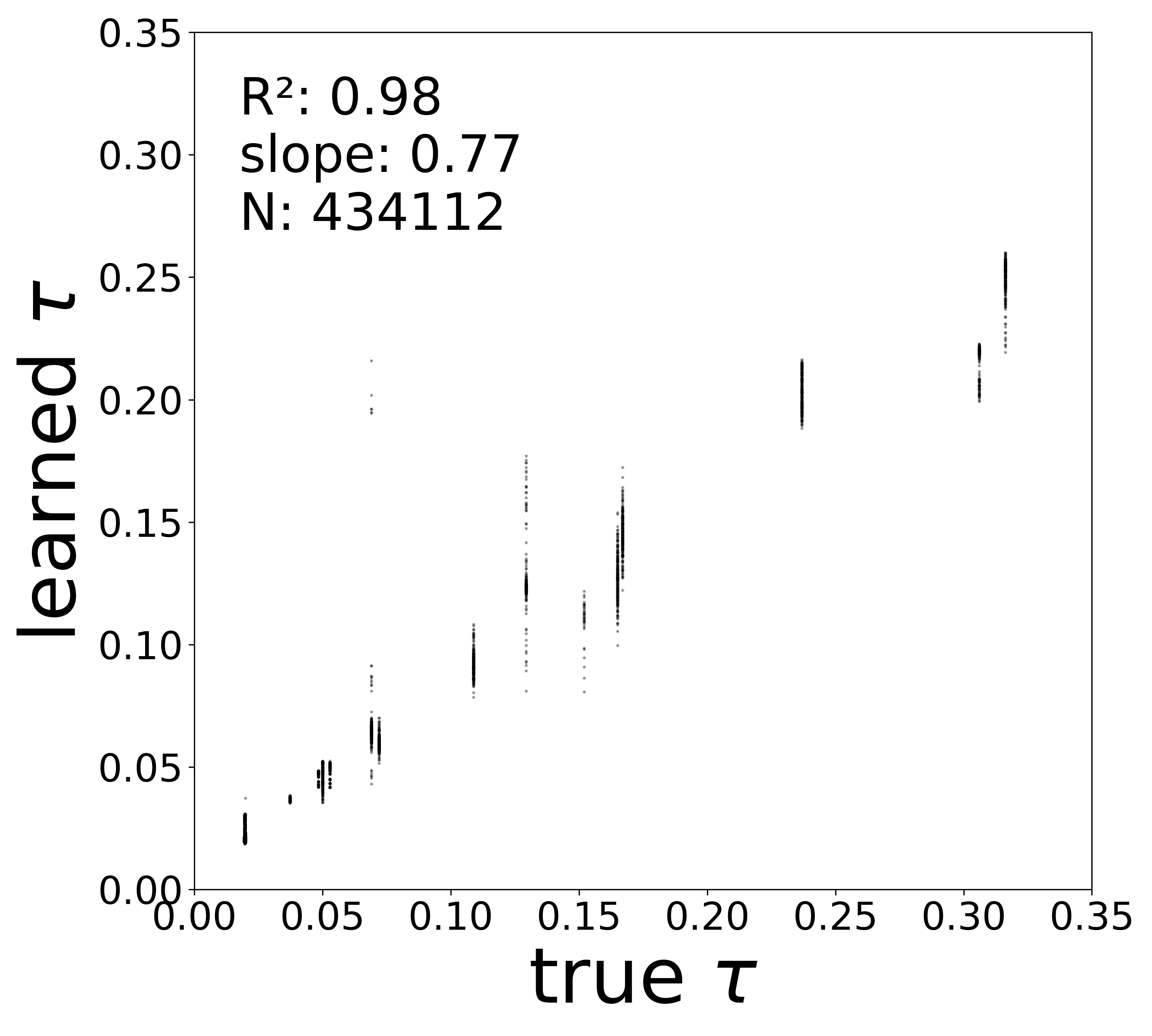
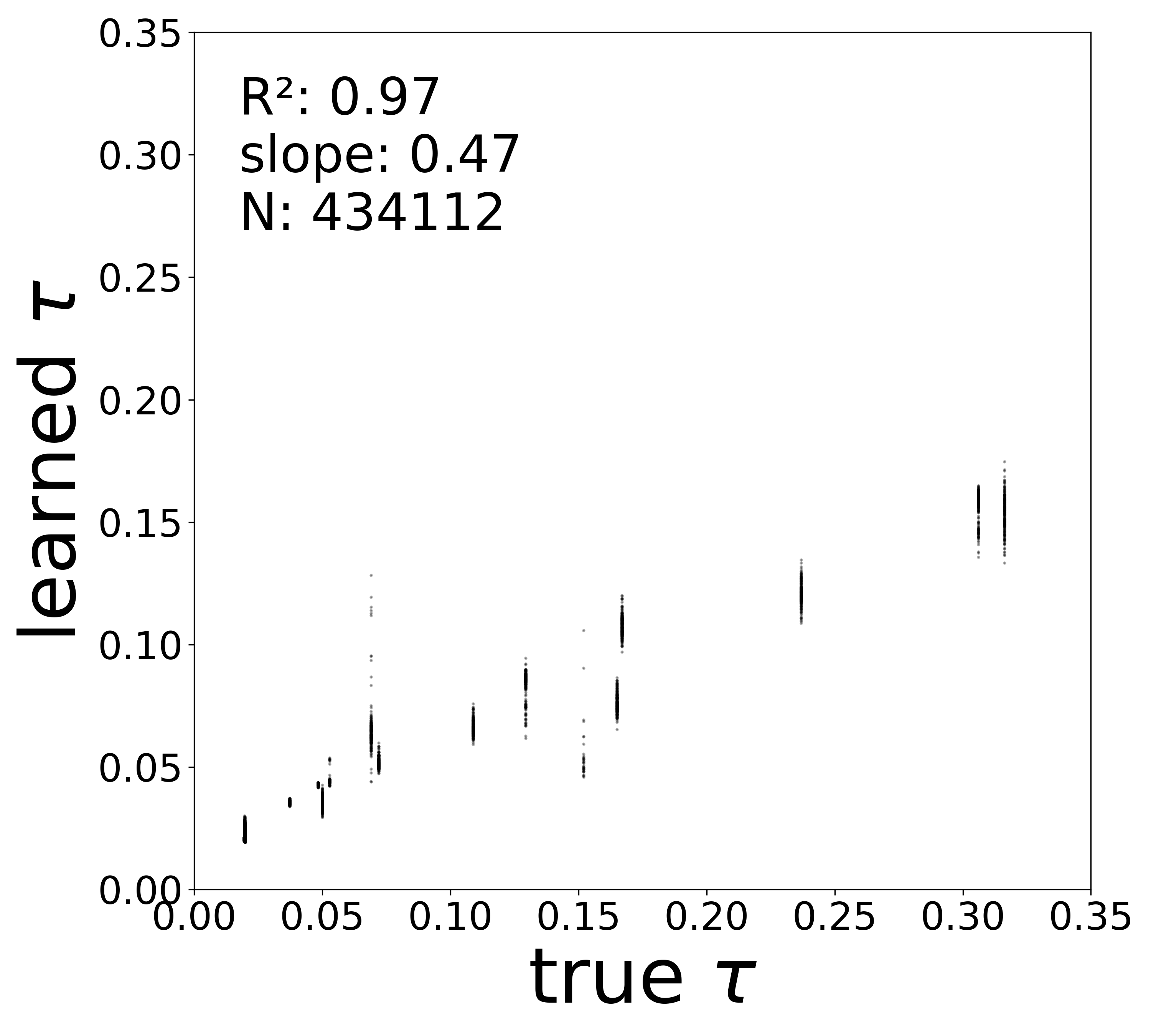
Synaptic weight recovery decreases from \(R^2 = 0.96\) at \(\sigma_{\text{meas}} = 0.02\) to \(0.76\) at \(\sigma_{\text{meas}} = 0.10\), while time constants remain robust (\(R^2 > 0.85\) across all conditions). Resting potentials are the most sensitive to measurement noise, dropping below \(R^2 = 0.05\) for \(\sigma_{\text{meas}} \geq 0.06\), consistent with the \(\sim 1/\Delta t\) amplification of noise in the derivative targets that \(V^{\text{rest}}\) depends on.
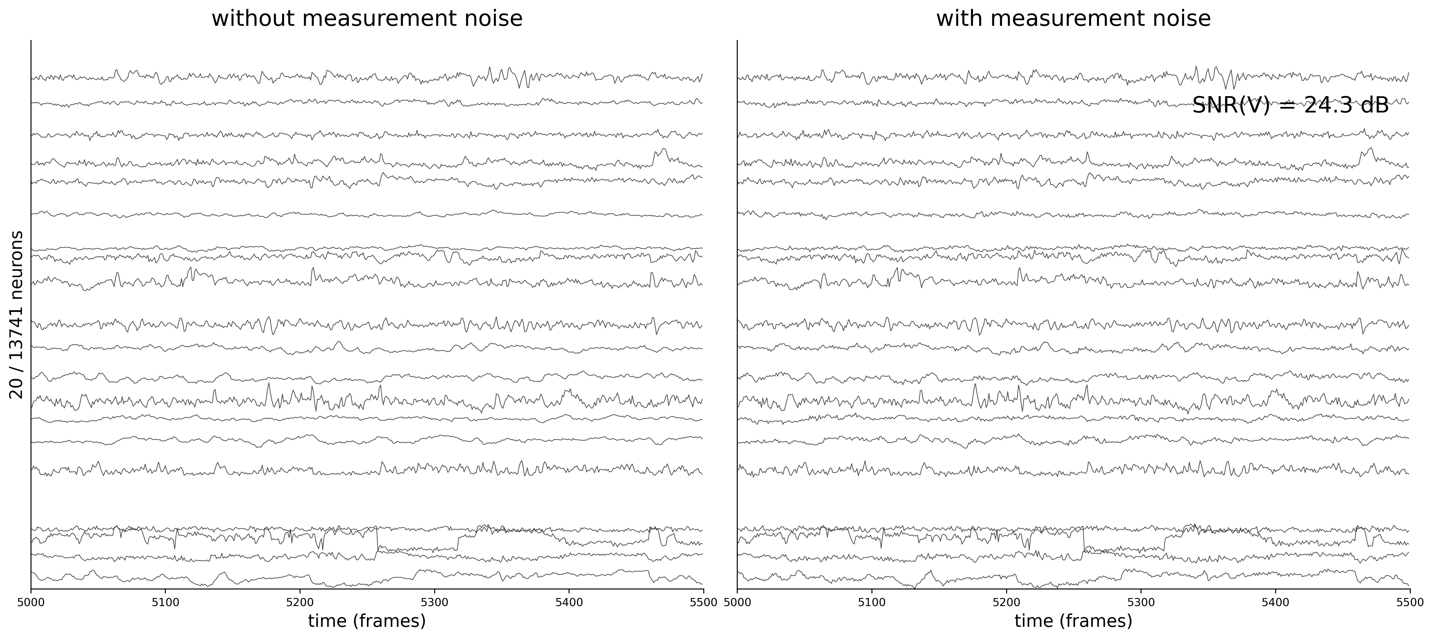
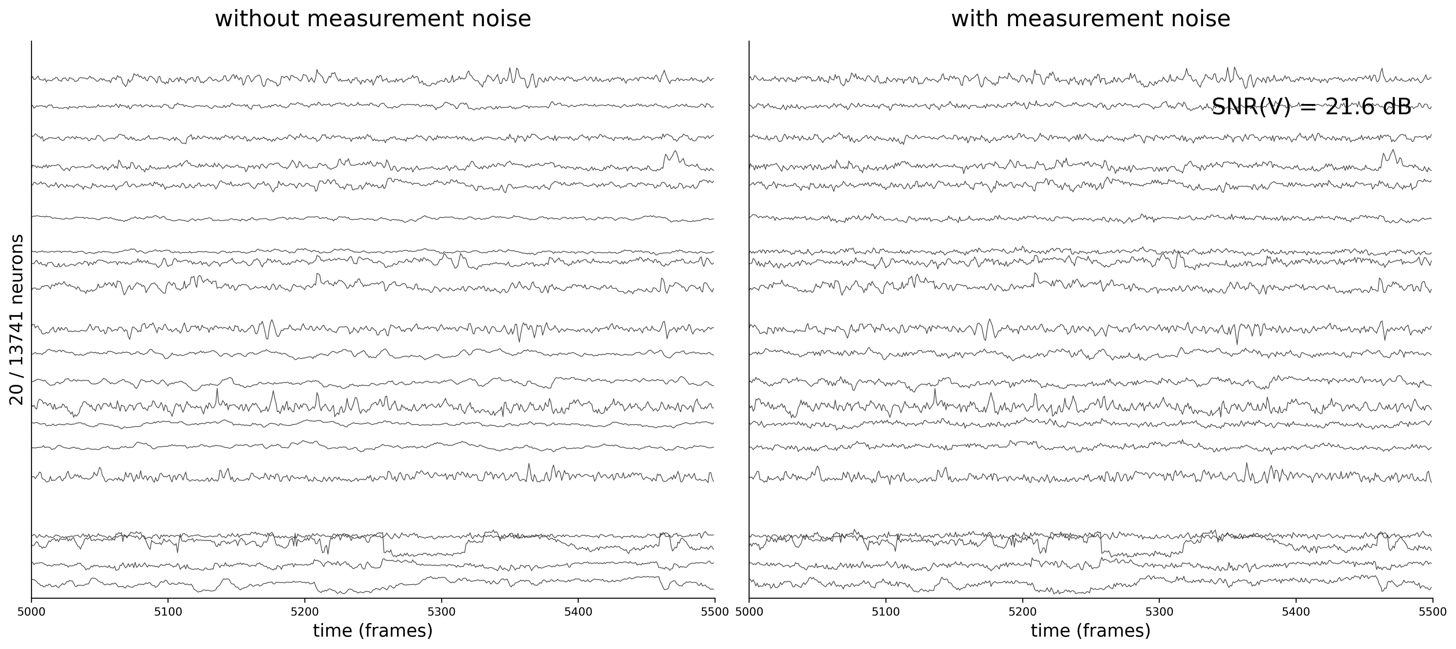
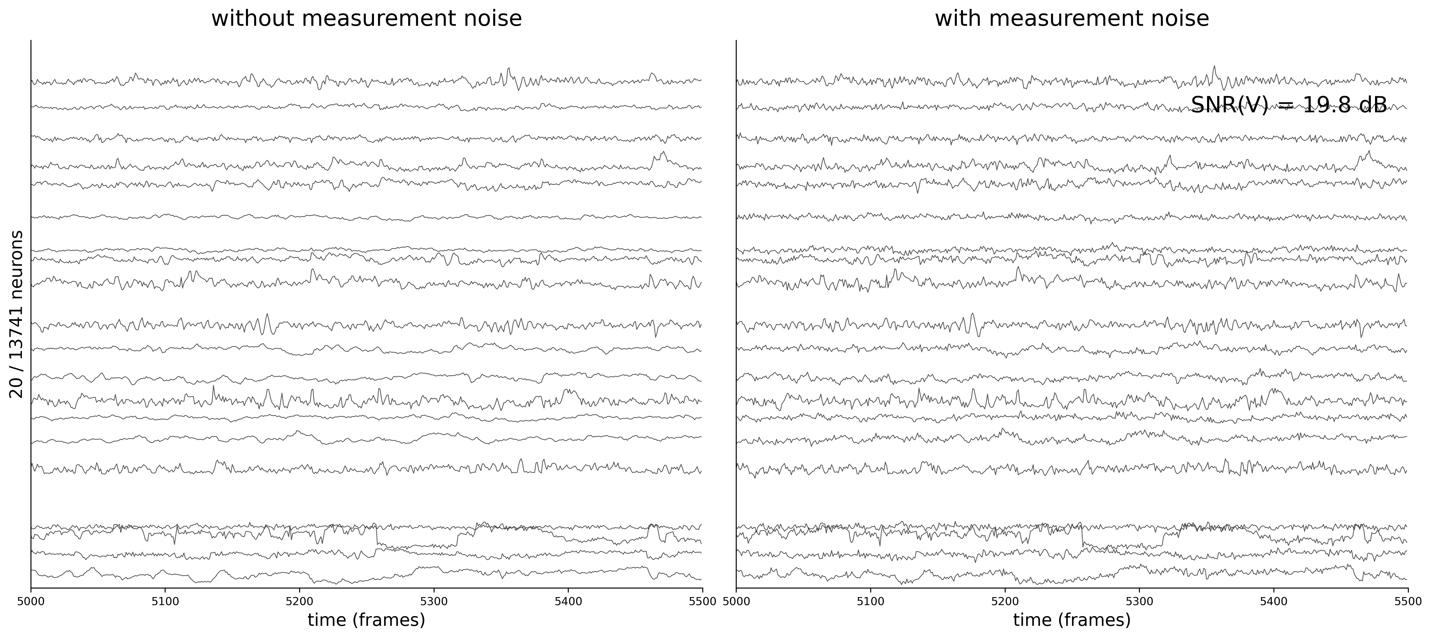
Activity Traces
Each figure shows 20 sampled neuron traces over a 500-frame window. The left panel displays the clean voltage from the ODE simulation (intrinsic dynamics noise \(\sigma_{\text{dyn}} = 0.05\) only).
The right panel shows the noisy observations \(\tilde{v}_i(t) = v_i(t) + \sigma_{\text{meas}}\,\eta_i(t)\) that the GNN actually receives during training. As \(\sigma_{\text{meas}}\) increases, the high-frequency measurement noise becomes clearly visible.
\(\sigma_{\text{meas}} = 0.02\)

\(\sigma_{\text{meas}} = 0.04\)

\(\sigma_{\text{meas}} = 0.06\)
\(\sigma_{\text{meas}} = 0.08\)
\(\sigma_{\text{meas}} = 0.10\)
Generate Analysis Plots
For each measurement noise condition, data_plot loads the best model checkpoint and generates the full suite of results visualizations.
Code
print()
print("=" * 80)
print("ANALYSIS - Generating results plots for all measurement noise conditions")
print("=" * 80)

for config_name, table_label, label in datasets:
    config = configs[config_name]
    print(f"\n--- {label} ---")
    data_plot(
        config=config,
        config_file=config.config_file,
        epoch_list=['best'],
        style='color',
        extended='plots',
        device=device,
    )
Connectivity Recovery
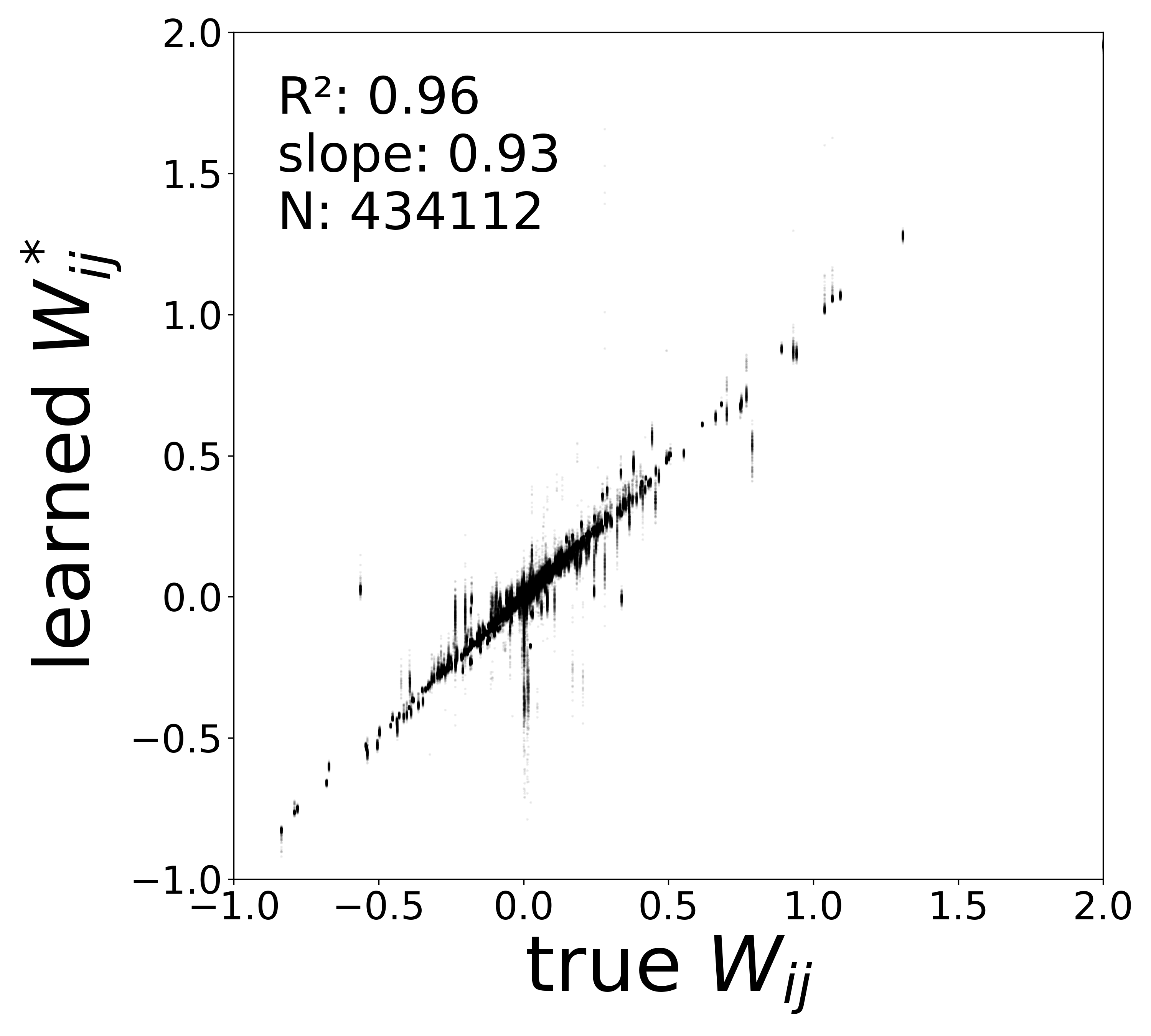
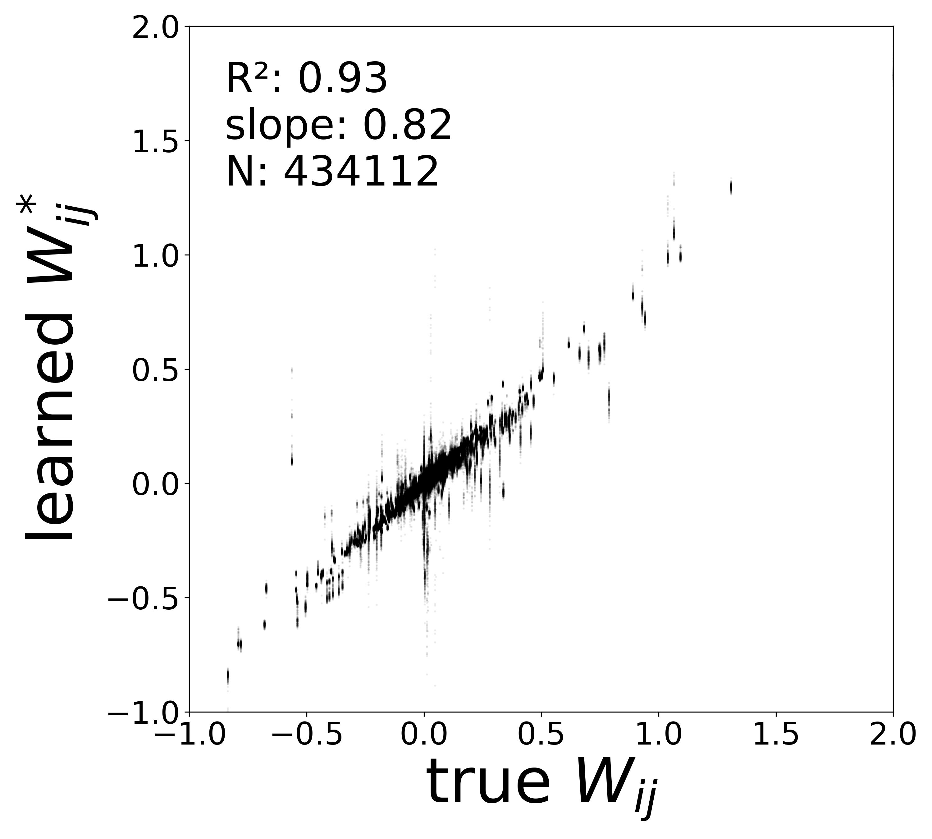
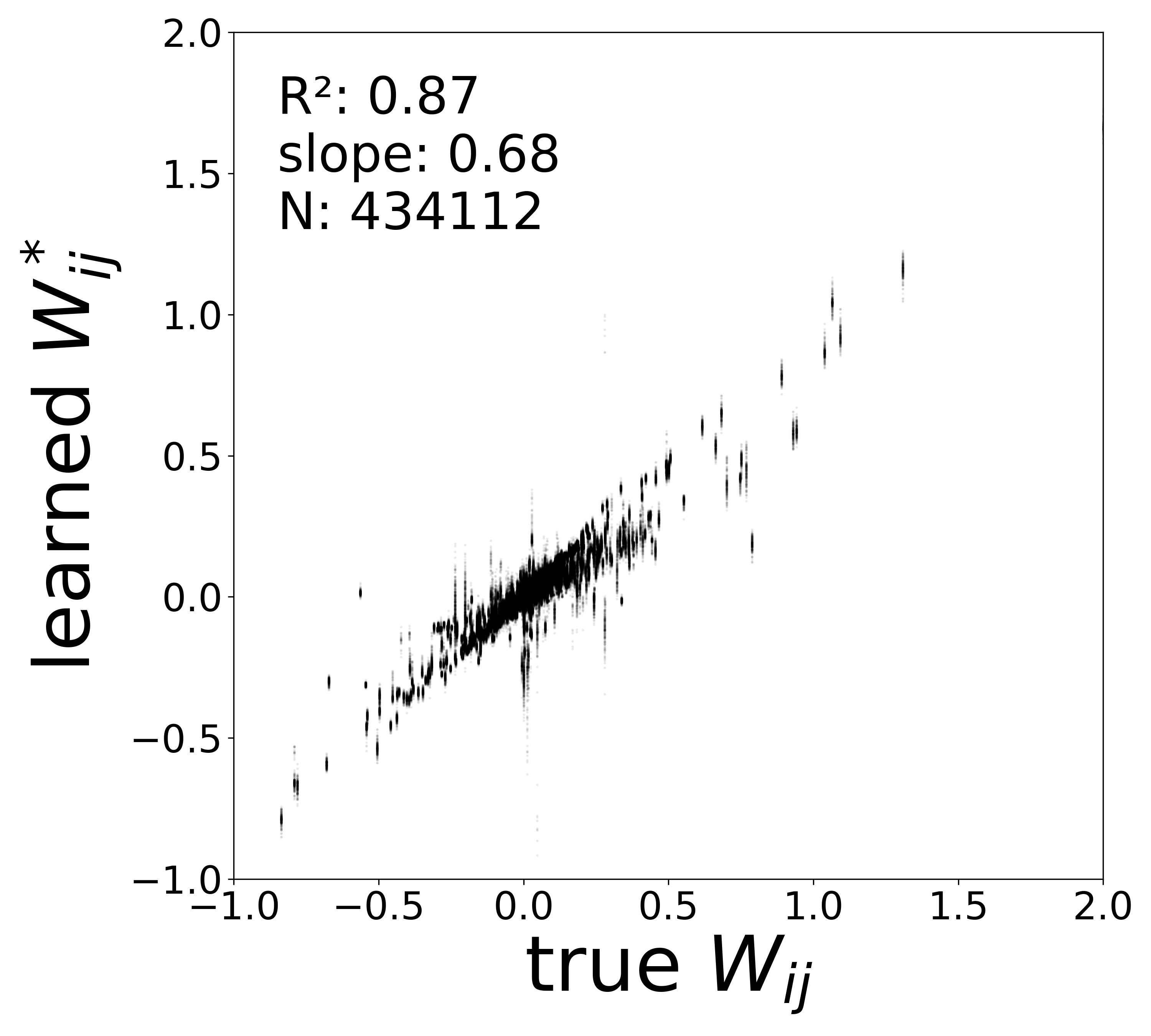
The scatter plots below compare the learned (corrected) synaptic weights \(W_{ij}^{\text{corr}}\) against the ground-truth connectome weights for all 434,112 edges. As measurement noise increases, the derivative targets become noisier and the weight recovery degrades.
\(\sigma_{\text{meas}} = 0.02\)
\(\sigma_{\text{meas}} = 0.04\)
\(\sigma_{\text{meas}} = 0.06\)
\(\sigma_{\text{meas}} = 0.08\)

\(\sigma_{\text{meas}} = 0.10\)

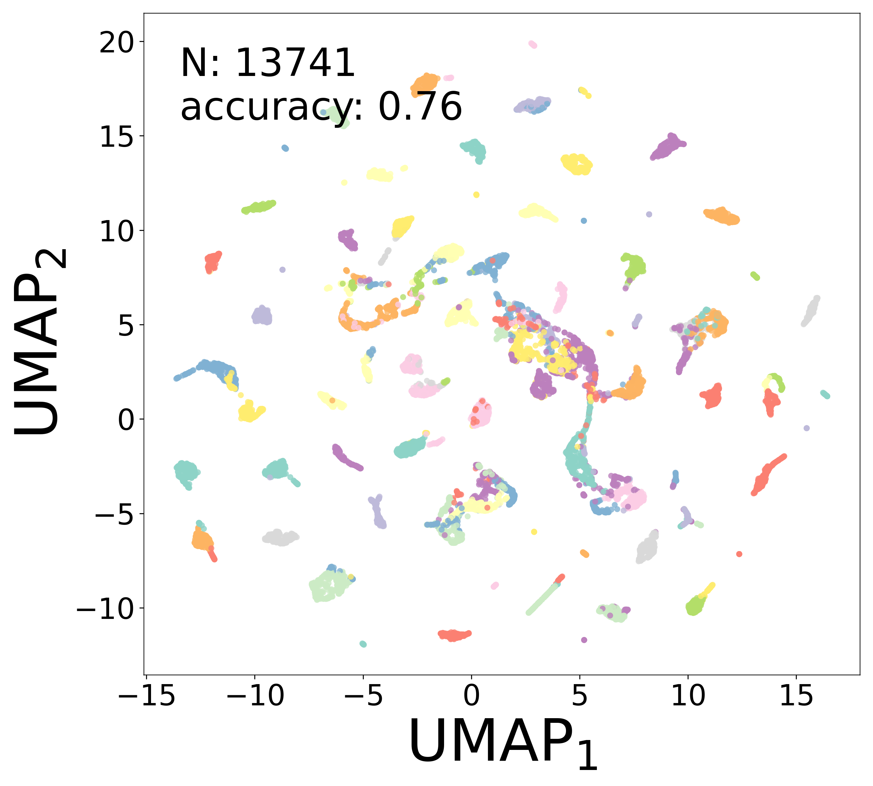
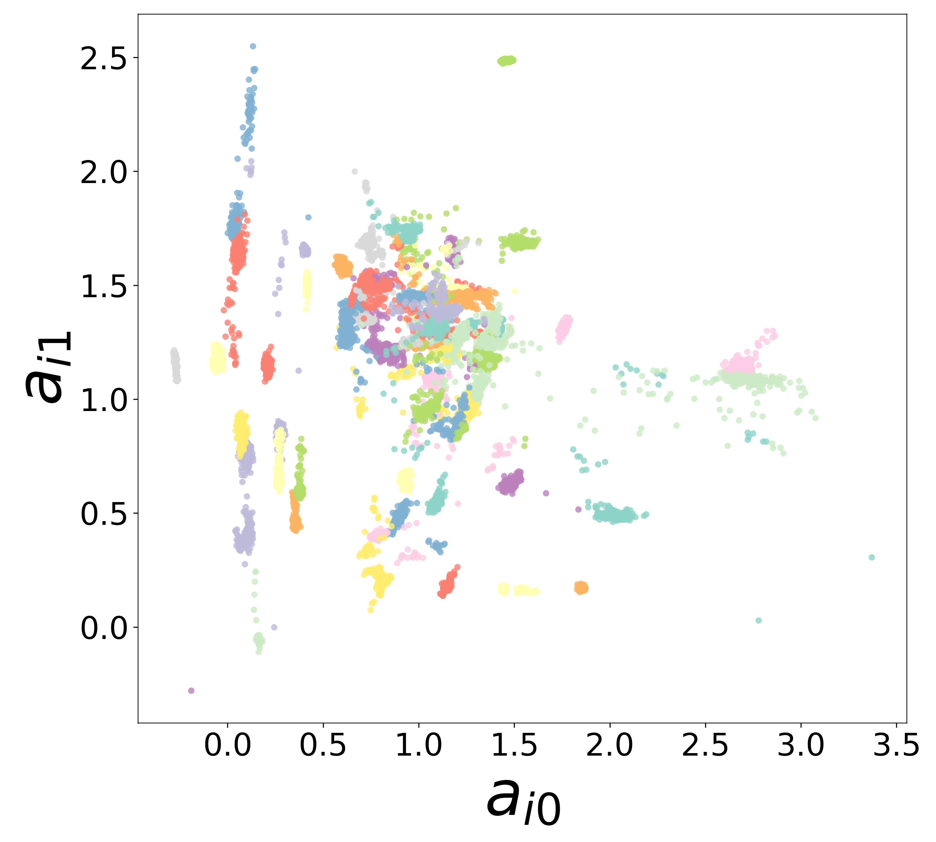
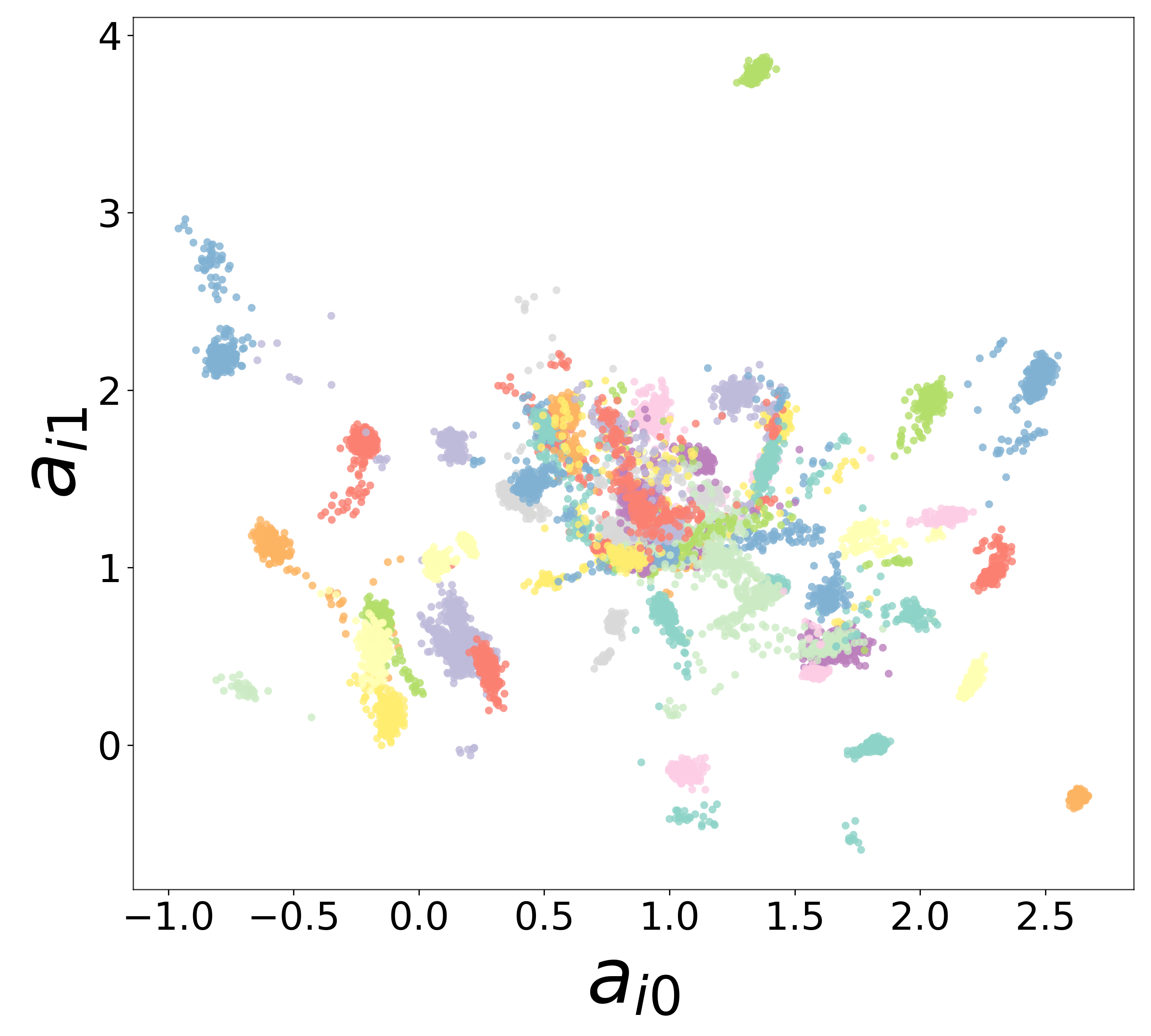
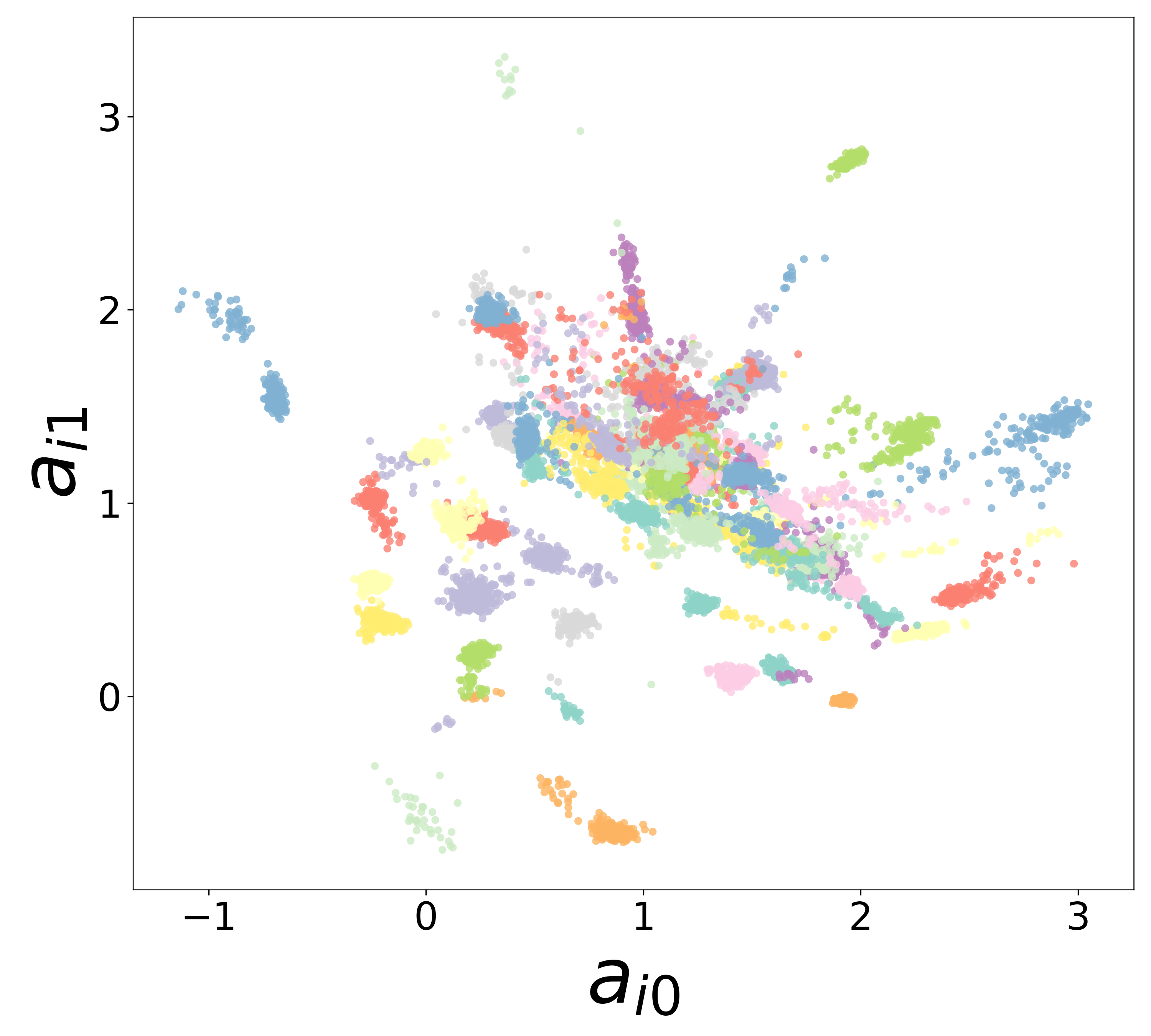
Neural Embeddings
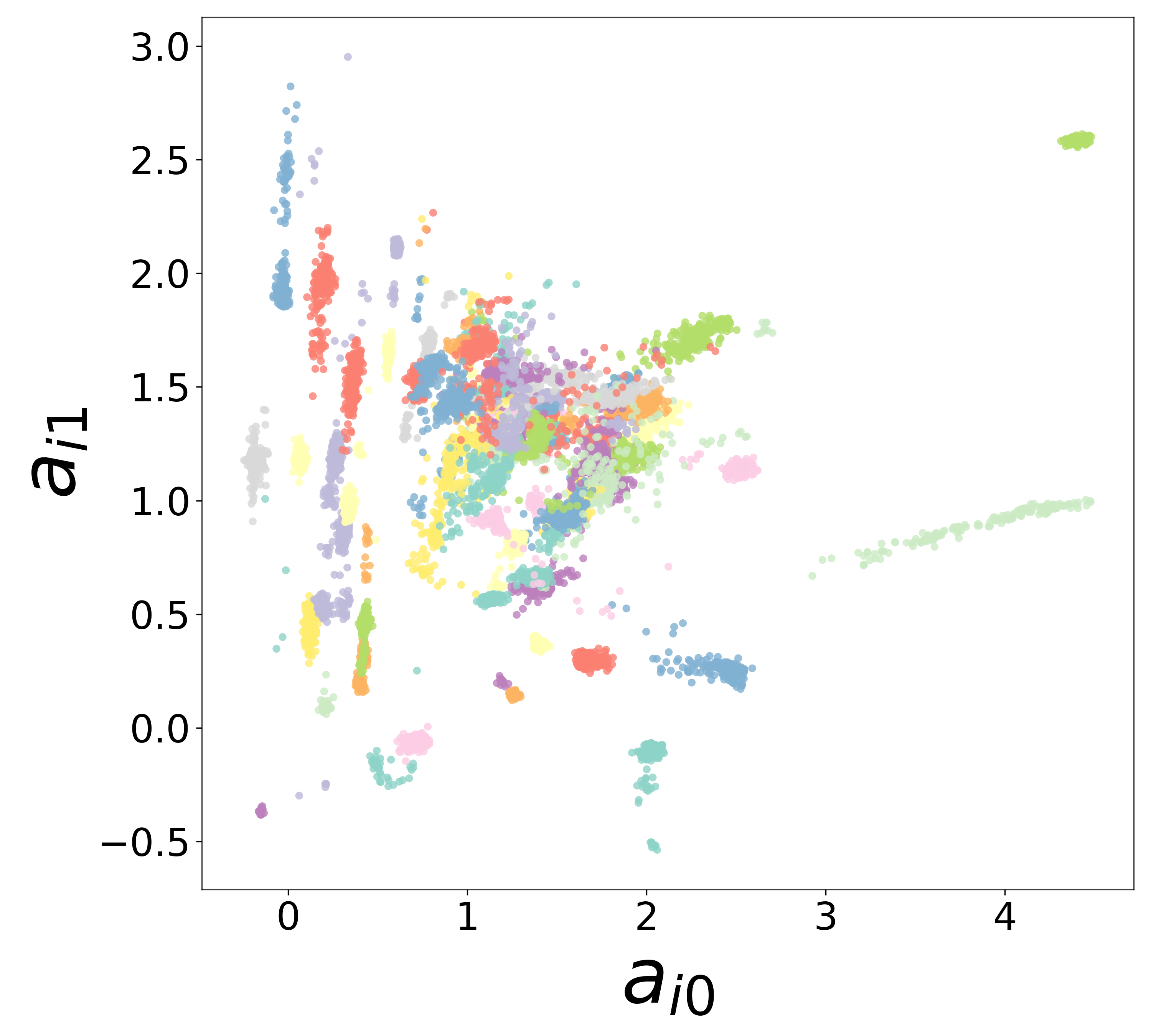
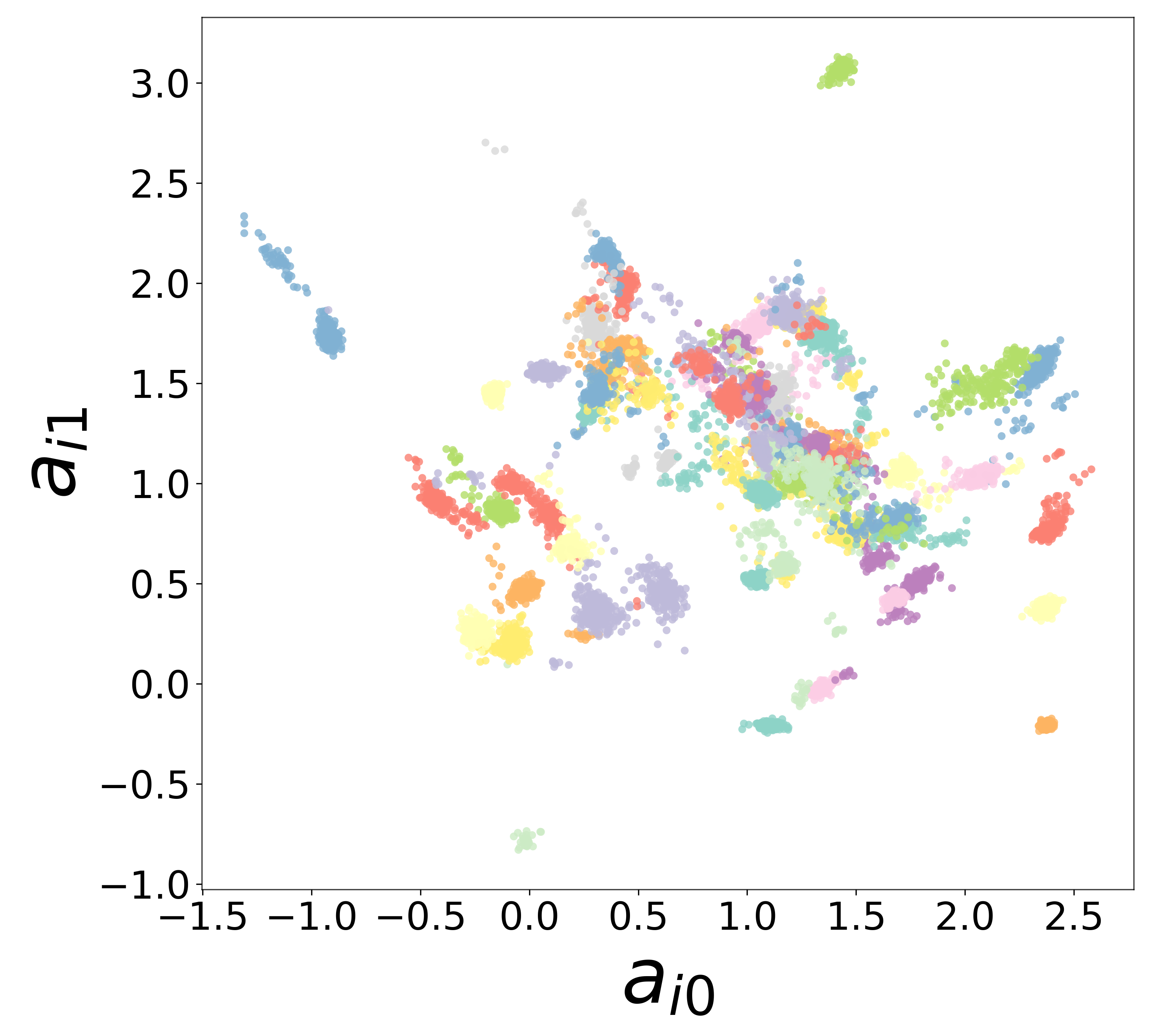
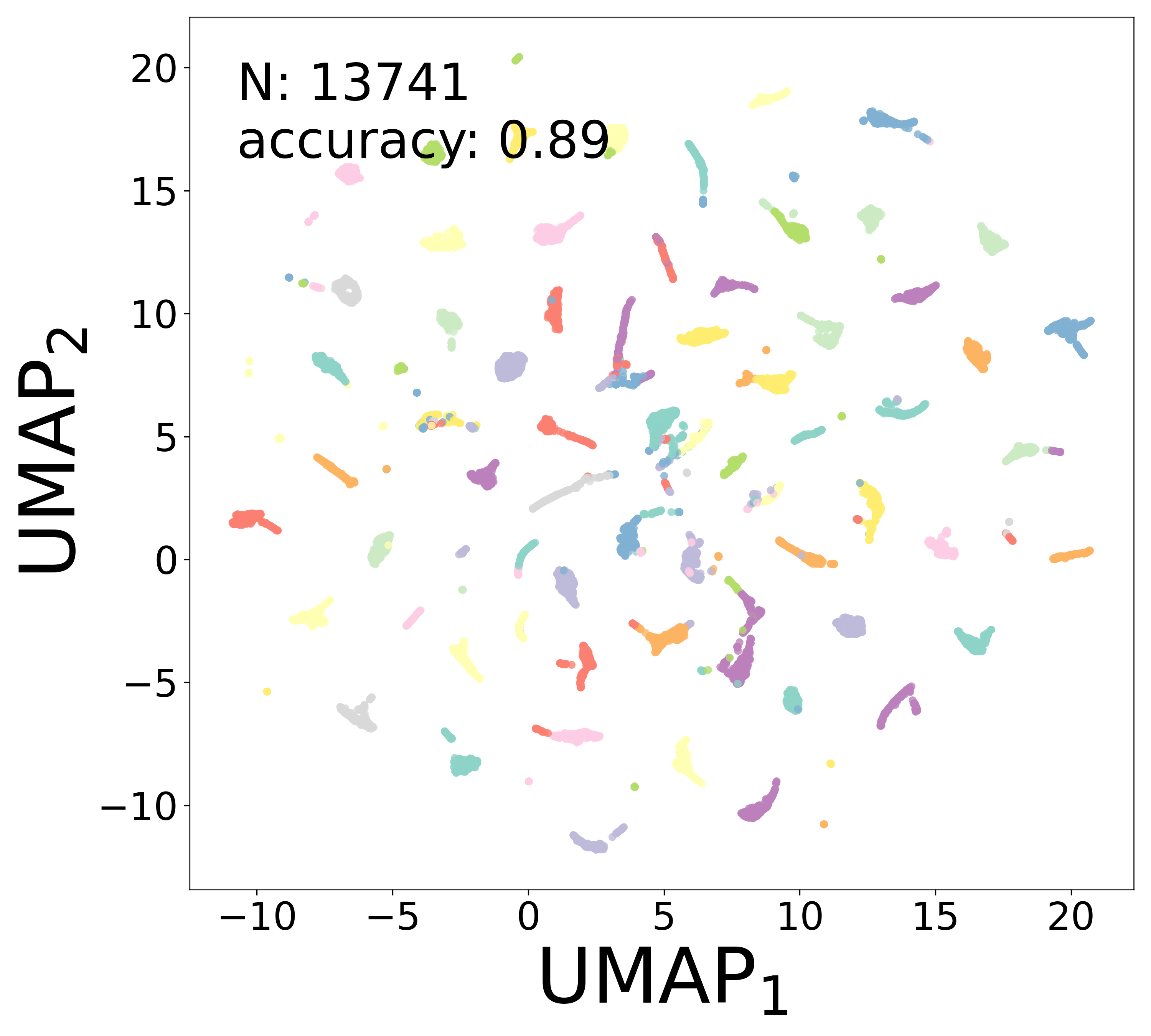
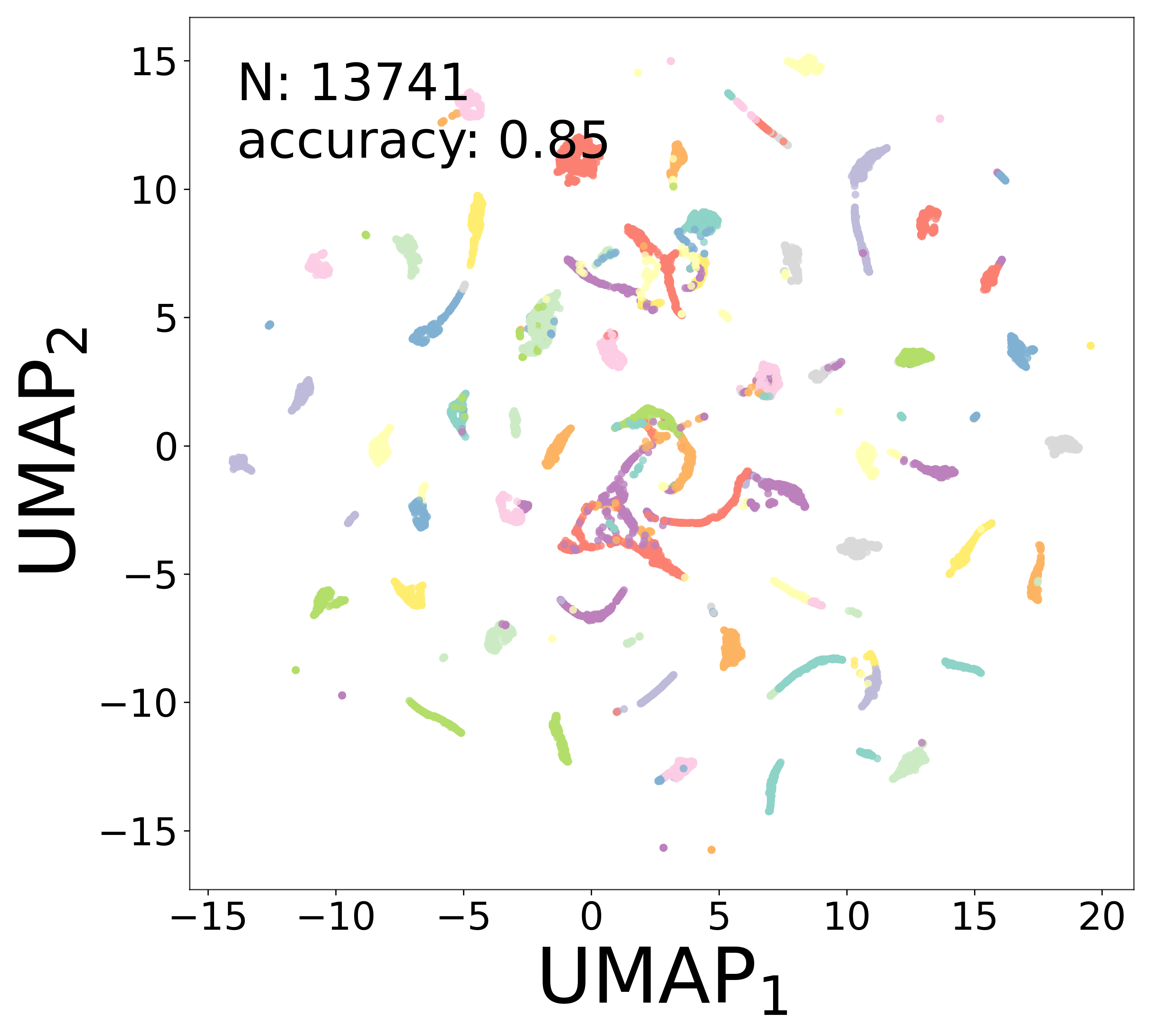
Each neuron is assigned a learned embedding \(\mathbf{a}_i\) that captures its functional identity. Tight clustering by cell type indicates that the GNN discovers neuron-type identity despite measurement noise.
\(\sigma_{\text{meas}} = 0.02\)

\(\sigma_{\text{meas}} = 0.04\)
\(\sigma_{\text{meas}} = 0.06\)

\(\sigma_{\text{meas}} = 0.08\)
\(\sigma_{\text{meas}} = 0.10\)

UMAP Projections
\(\sigma_{\text{meas}} = 0.02\)
\(\sigma_{\text{meas}} = 0.04\)
\(\sigma_{\text{meas}} = 0.06\)
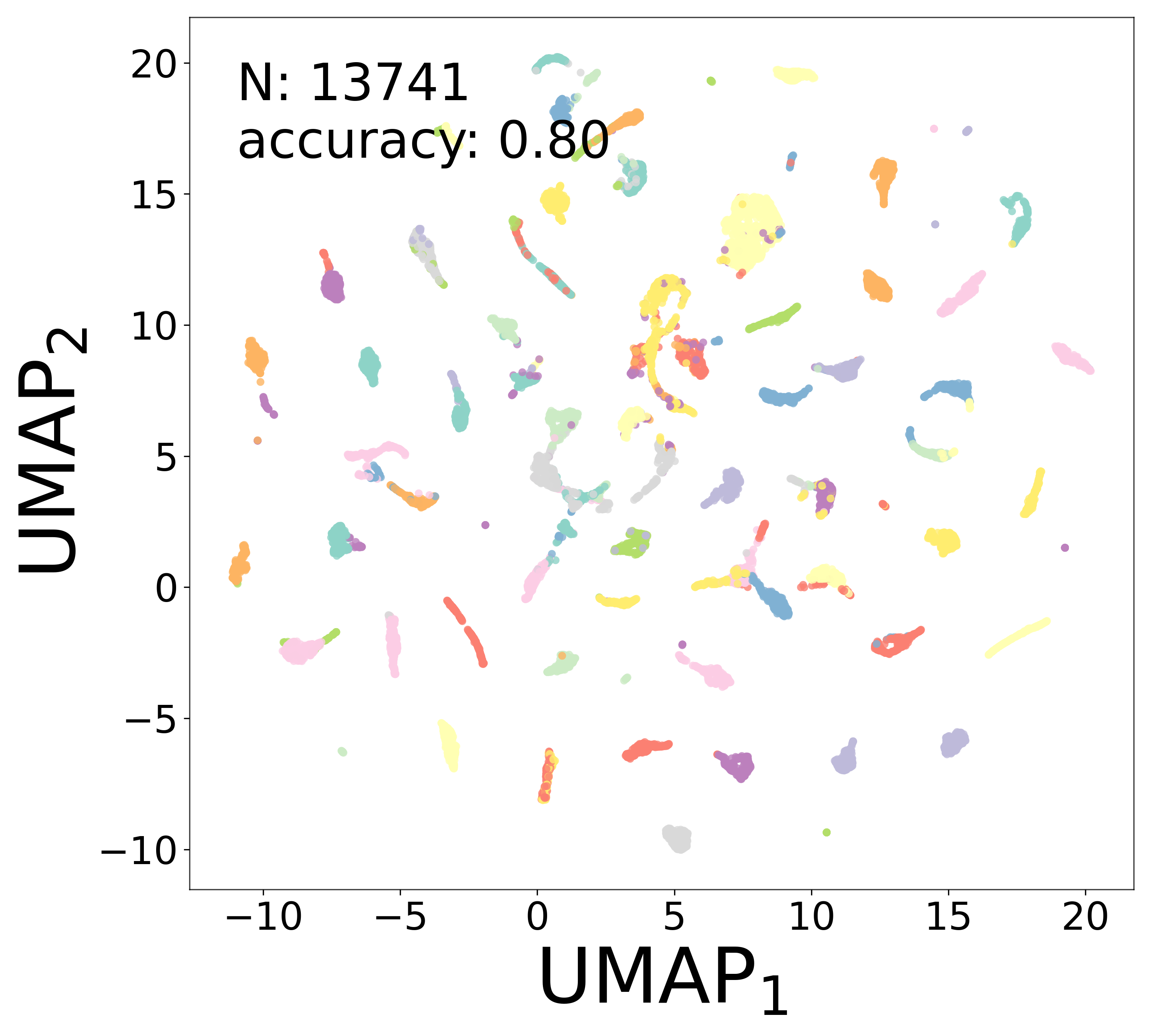
\(\sigma_{\text{meas}} = 0.08\)
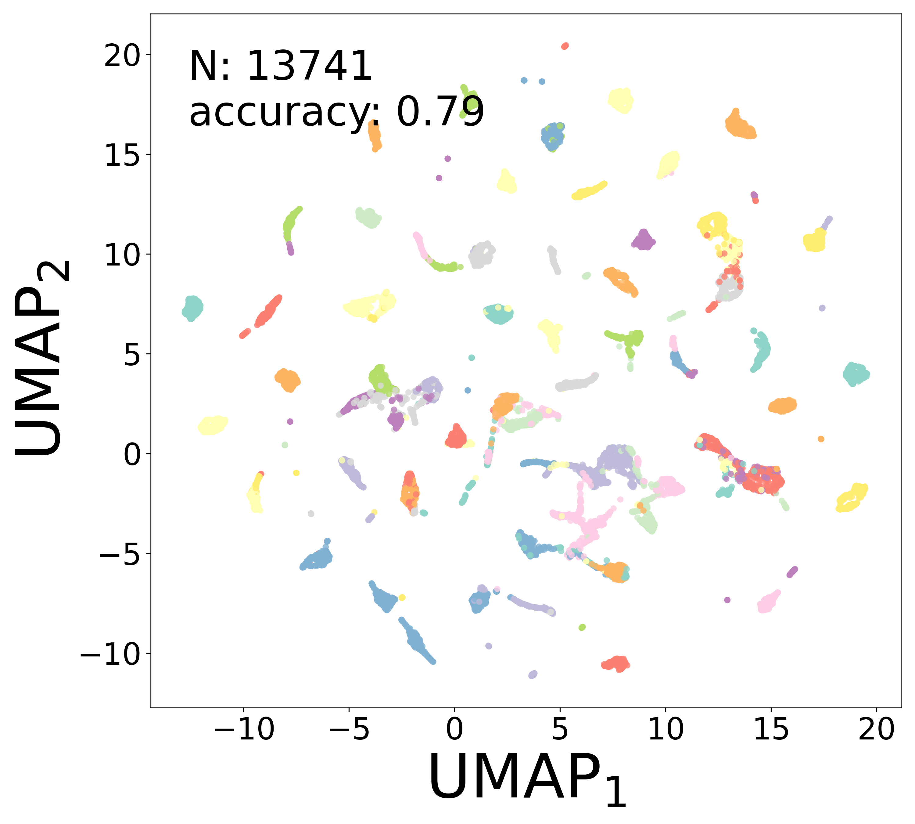
\(\sigma_{\text{meas}} = 0.10\)
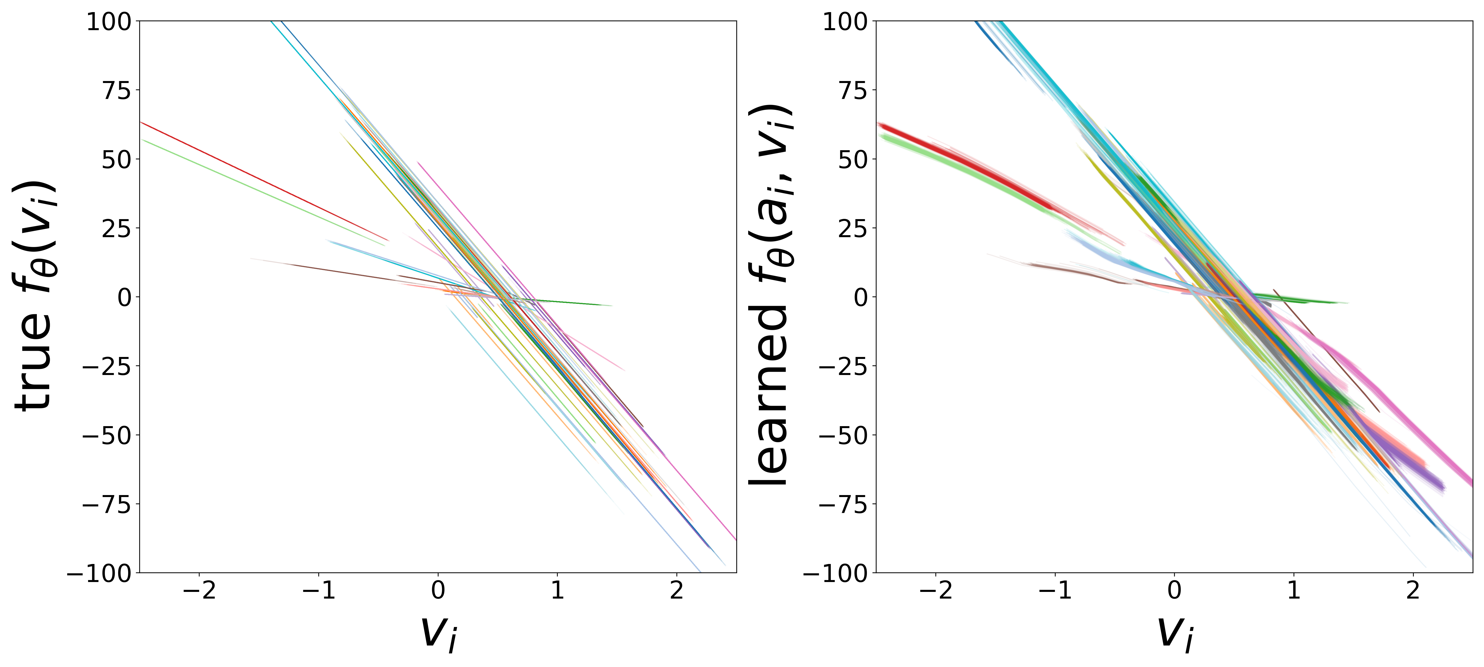
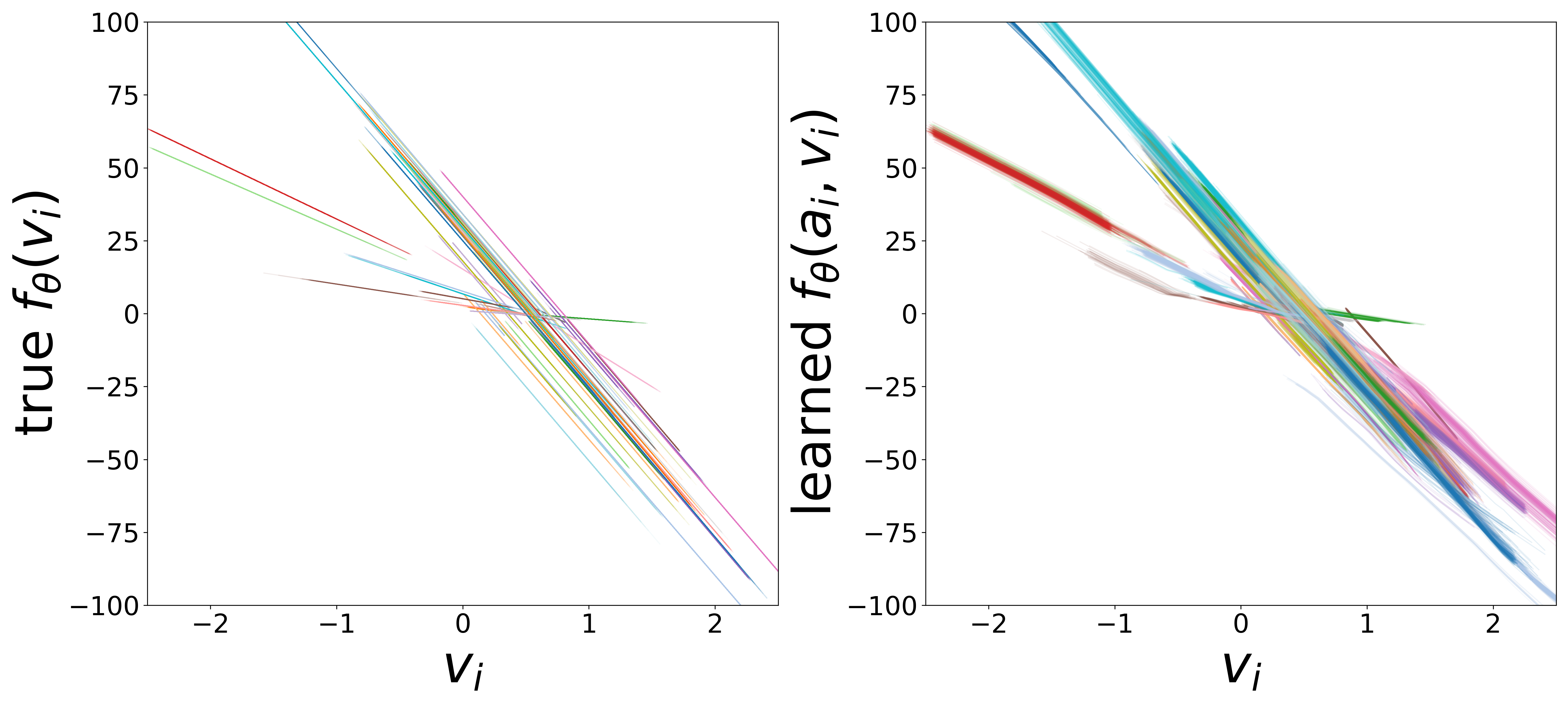
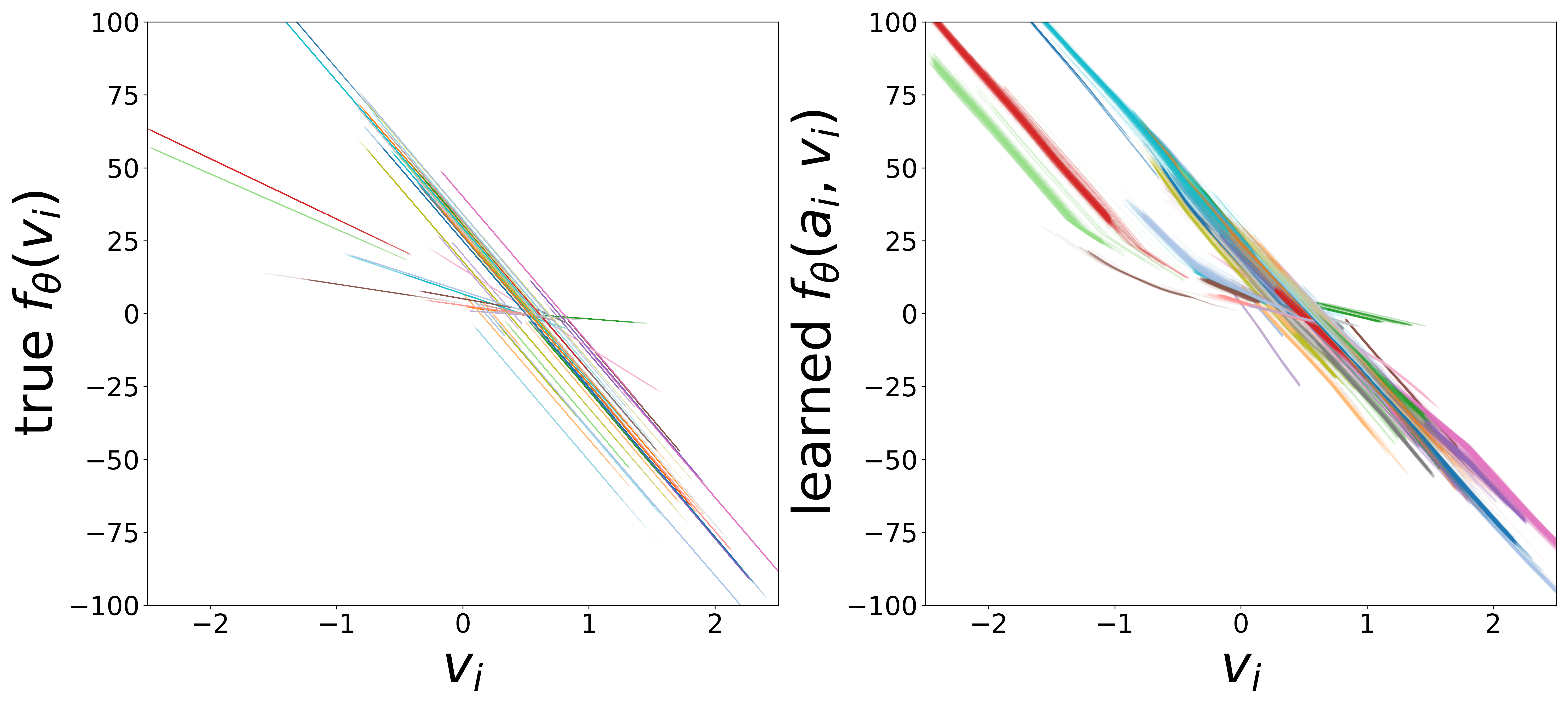
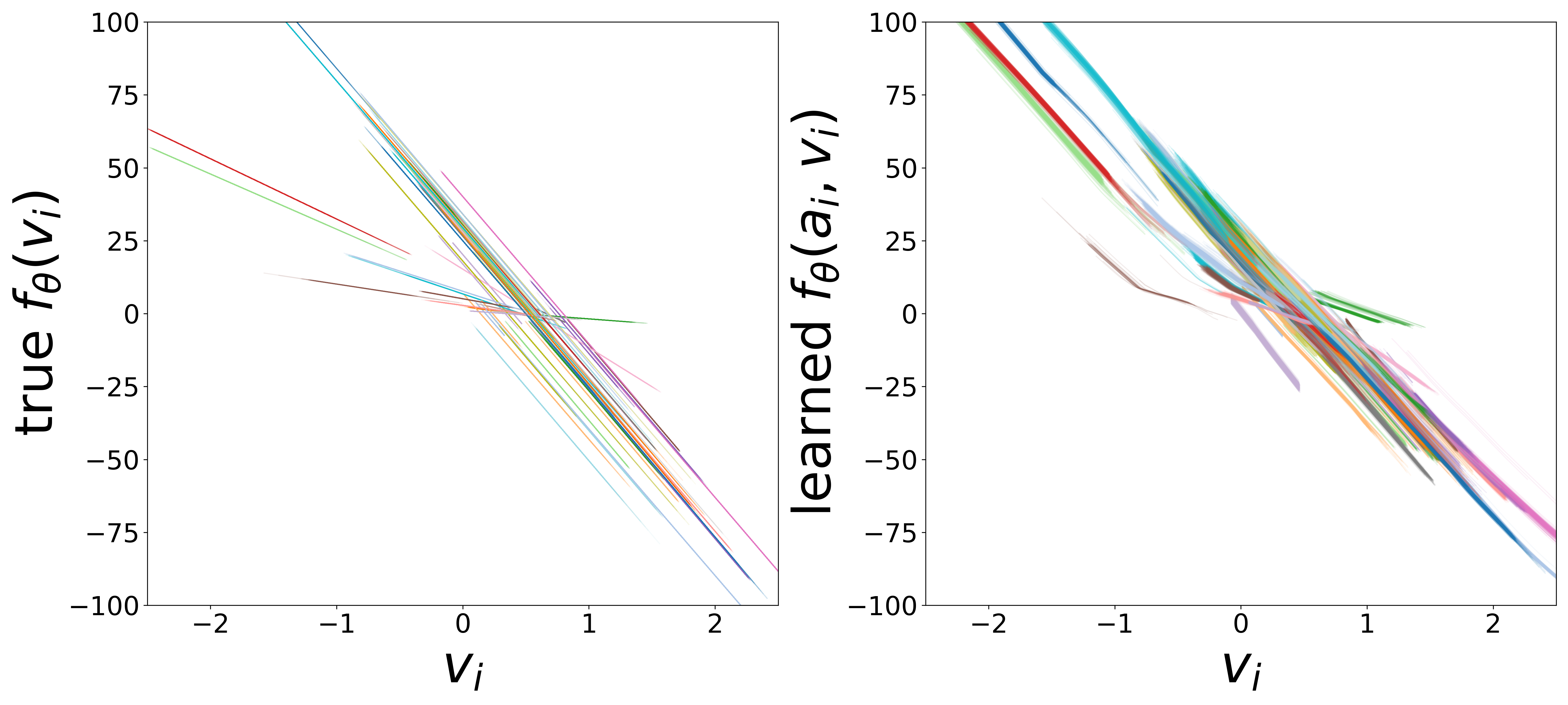
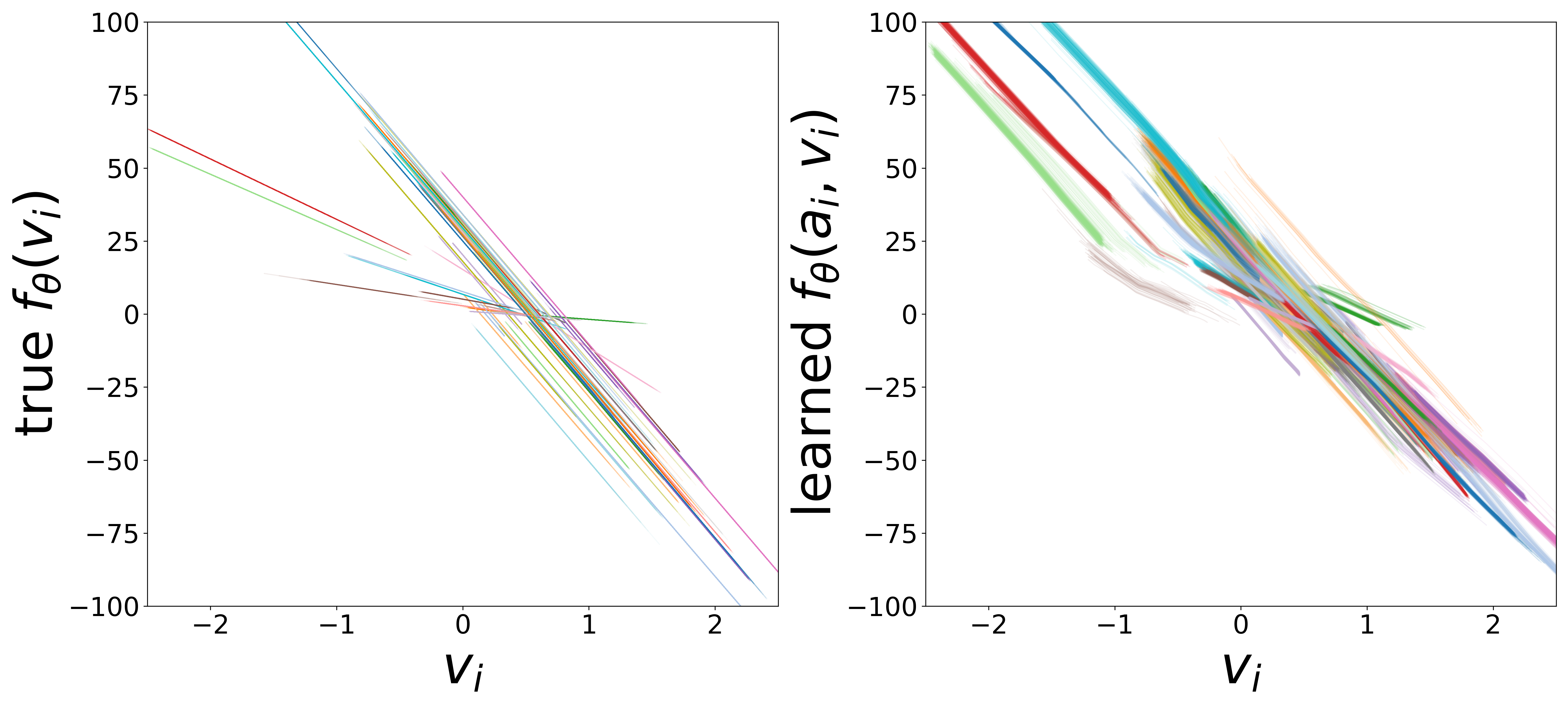
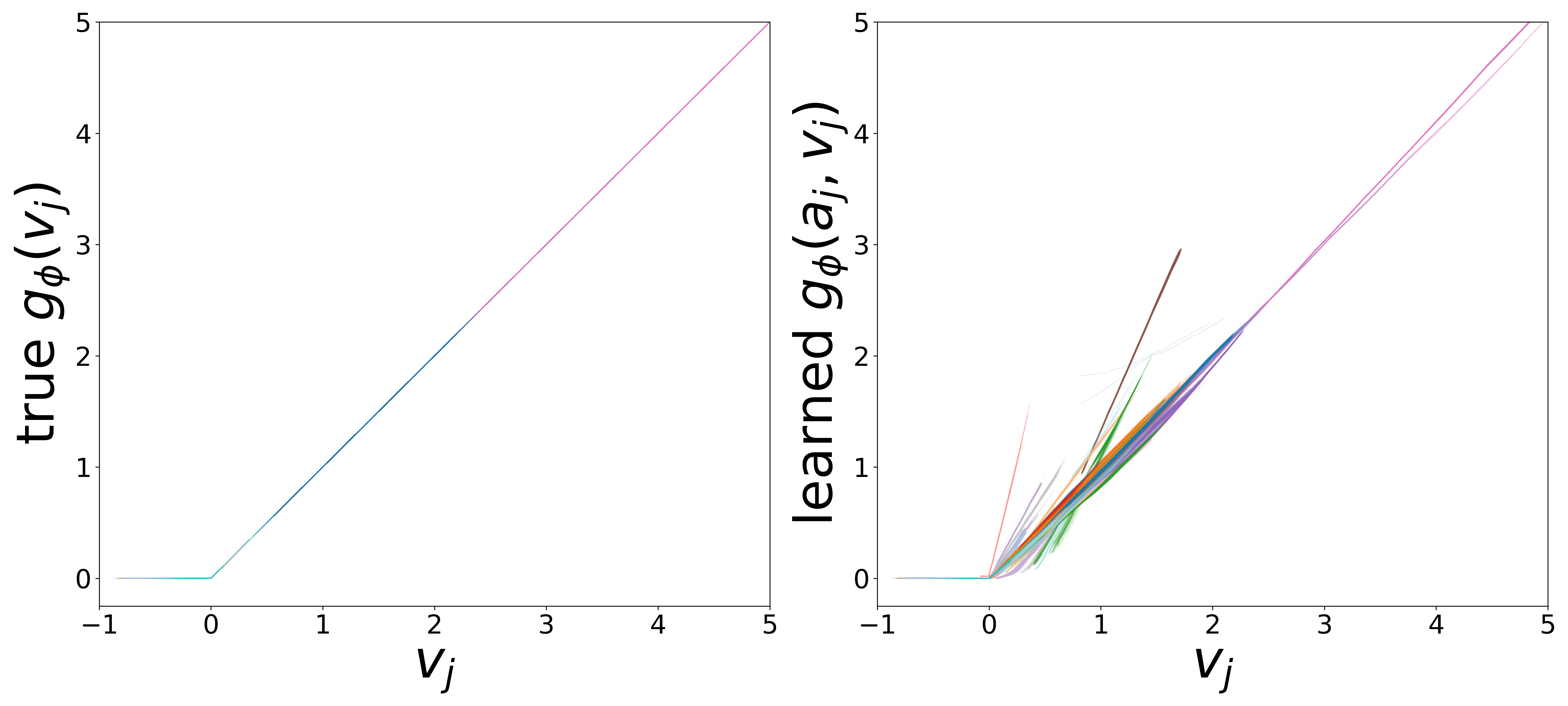
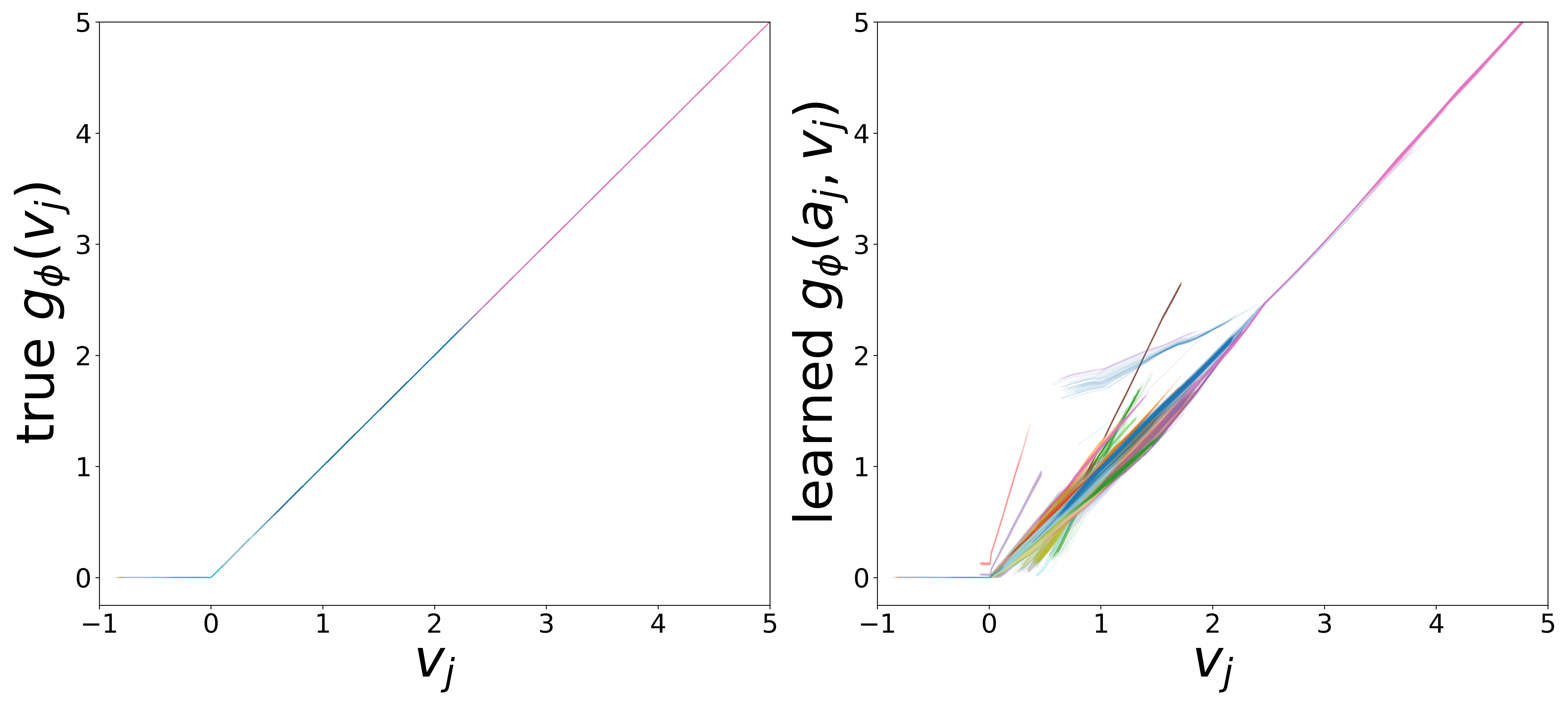
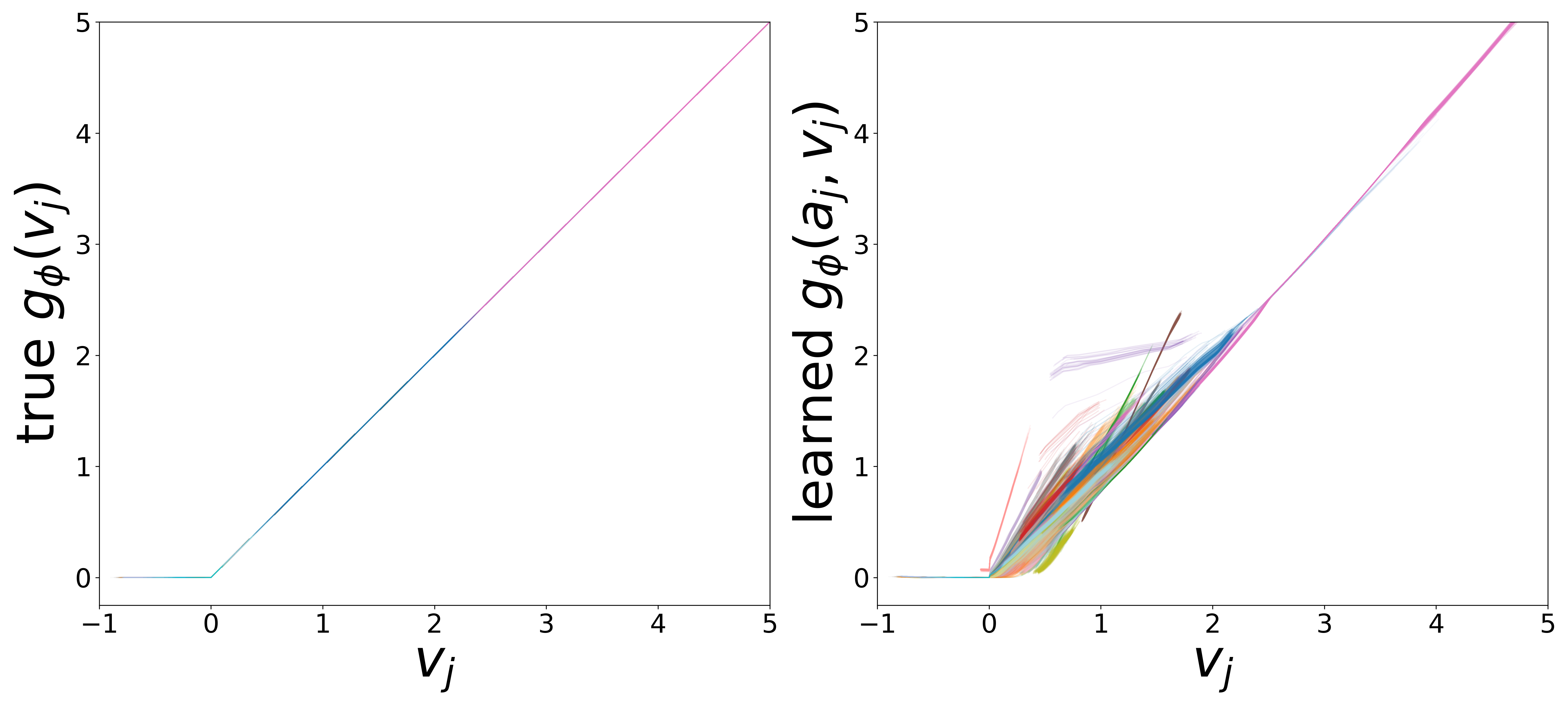
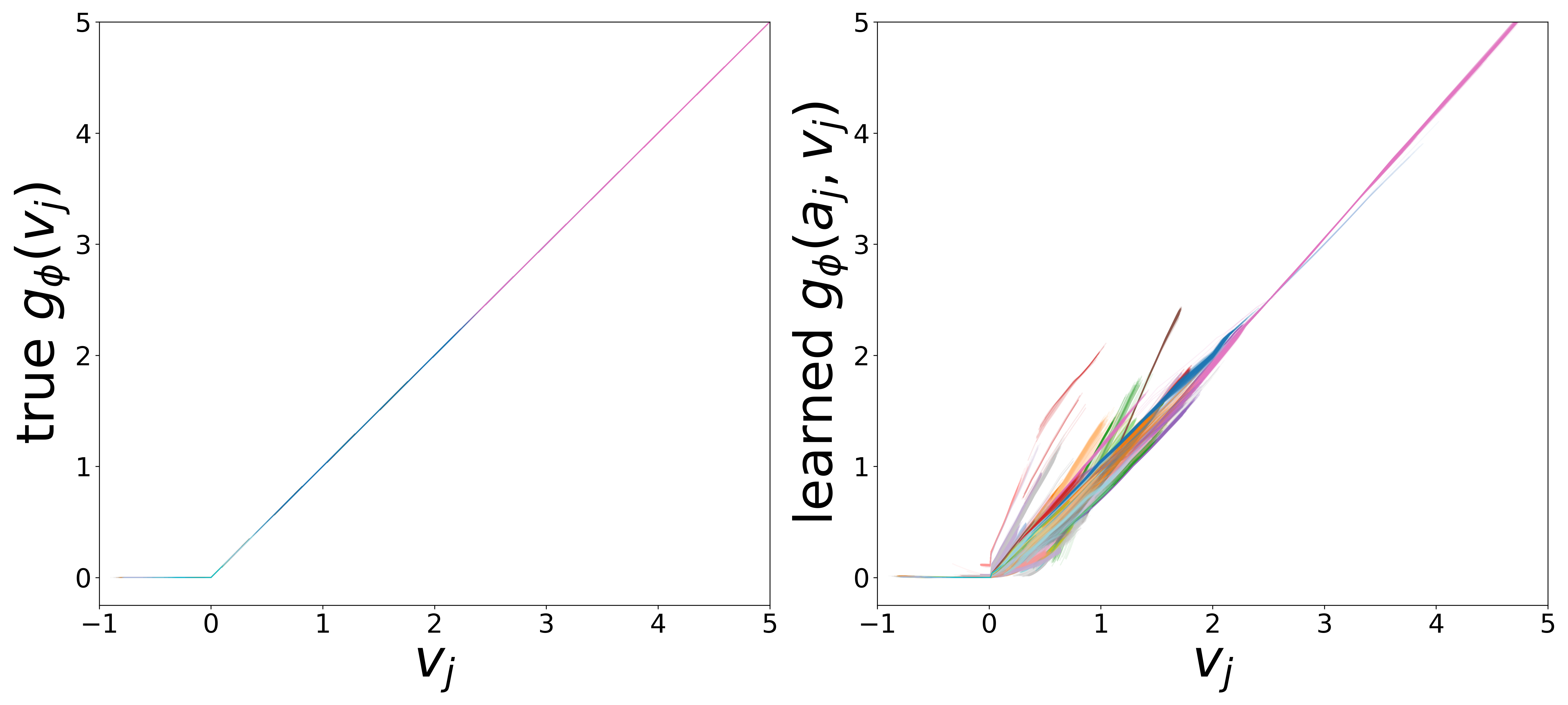
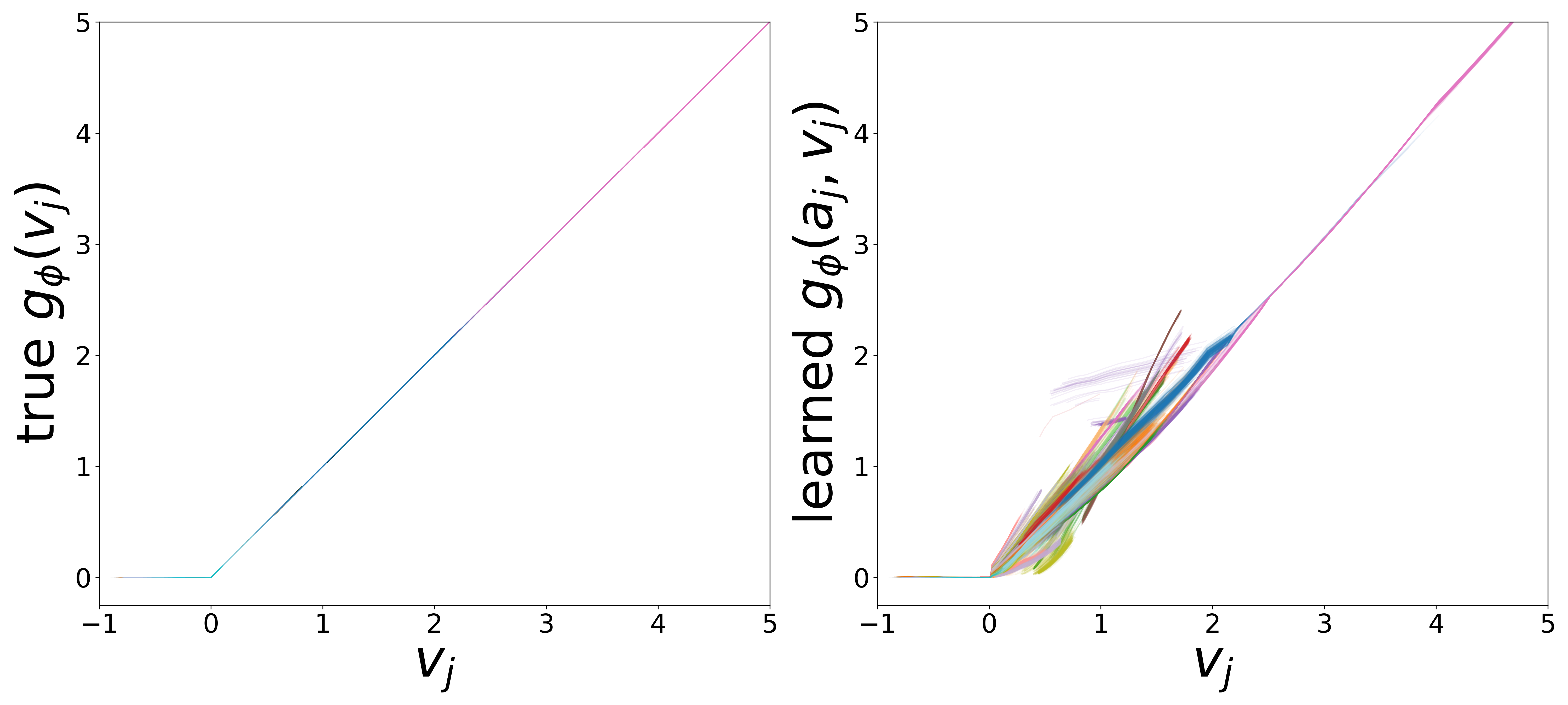
Learned Functions
The domain-restricted plots show the true ground-truth function (left panel) alongside the learned function (right panel) for each measurement noise condition. As noise increases, the learned functions deviate more from the ground truth, but the overall shape is often preserved.
\(f_\theta\) (MLP\(_0\)): Neuron Update Function
\(\sigma_{\text{meas}} = 0.02\)
\(\sigma_{\text{meas}} = 0.04\)
\(\sigma_{\text{meas}} = 0.06\)
\(\sigma_{\text{meas}} = 0.08\)
\(\sigma_{\text{meas}} = 0.10\)
Time Constants (\(\tau\))
\(\sigma_{\text{meas}} = 0.02\)
\(\sigma_{\text{meas}} = 0.04\)
\(\sigma_{\text{meas}} = 0.06\)
\(\sigma_{\text{meas}} = 0.08\)

\(\sigma_{\text{meas}} = 0.10\)
Resting Potentials (\(V^{\text{rest}}\))
\(\sigma_{\text{meas}} = 0.02\)
\(\sigma_{\text{meas}} = 0.04\)
\(\sigma_{\text{meas}} = 0.06\)
\(\sigma_{\text{meas}} = 0.08\)
\(\sigma_{\text{meas}} = 0.10\)
\(g_\phi\) (MLP\(_1\)): Edge Message Function
\(\sigma_{\text{meas}} = 0.02\)
\(\sigma_{\text{meas}} = 0.04\)
\(\sigma_{\text{meas}} = 0.06\)
\(\sigma_{\text{meas}} = 0.08\)
\(\sigma_{\text{meas}} = 0.10\)
Neural Embeddings
\(\sigma_{\text{meas}} = 0.02\)
\(\sigma_{\text{meas}} = 0.04\)

\(\sigma_{\text{meas}} = 0.06\)
\(\sigma_{\text{meas}} = 0.08\)

\(\sigma_{\text{meas}} = 0.10\)
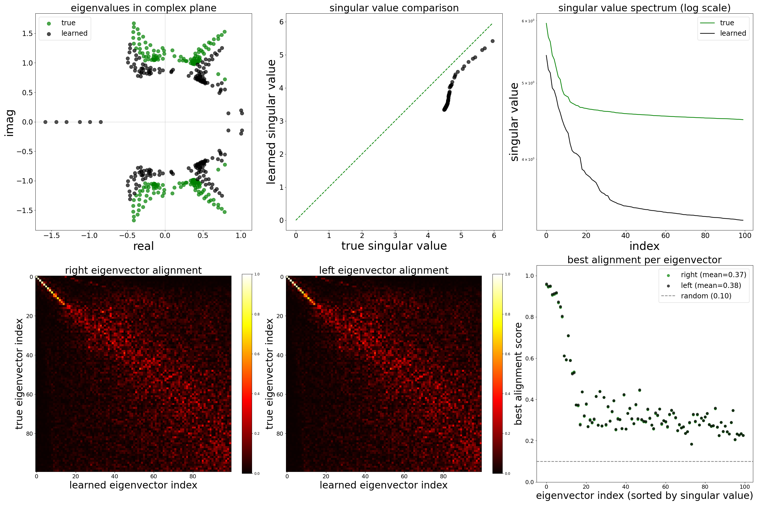
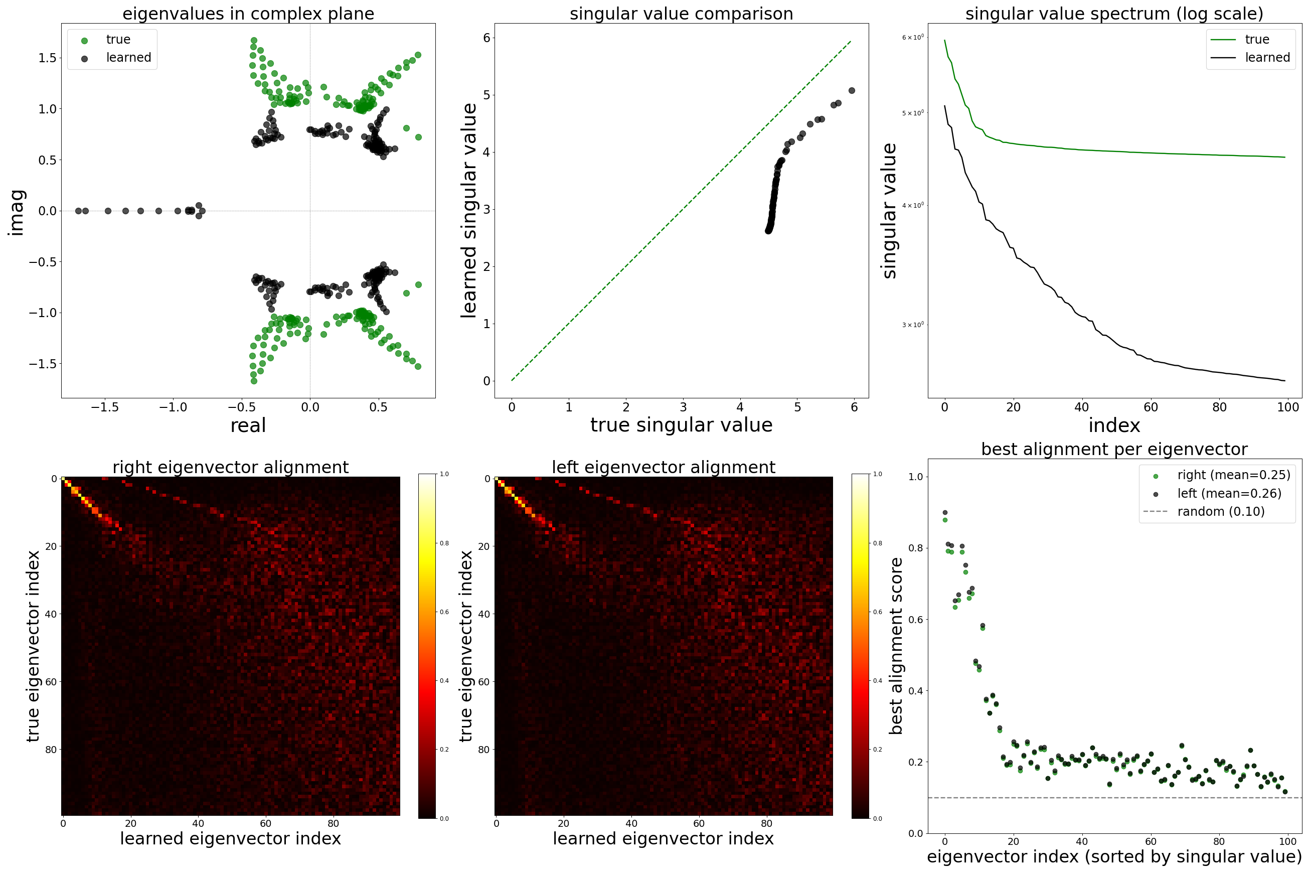
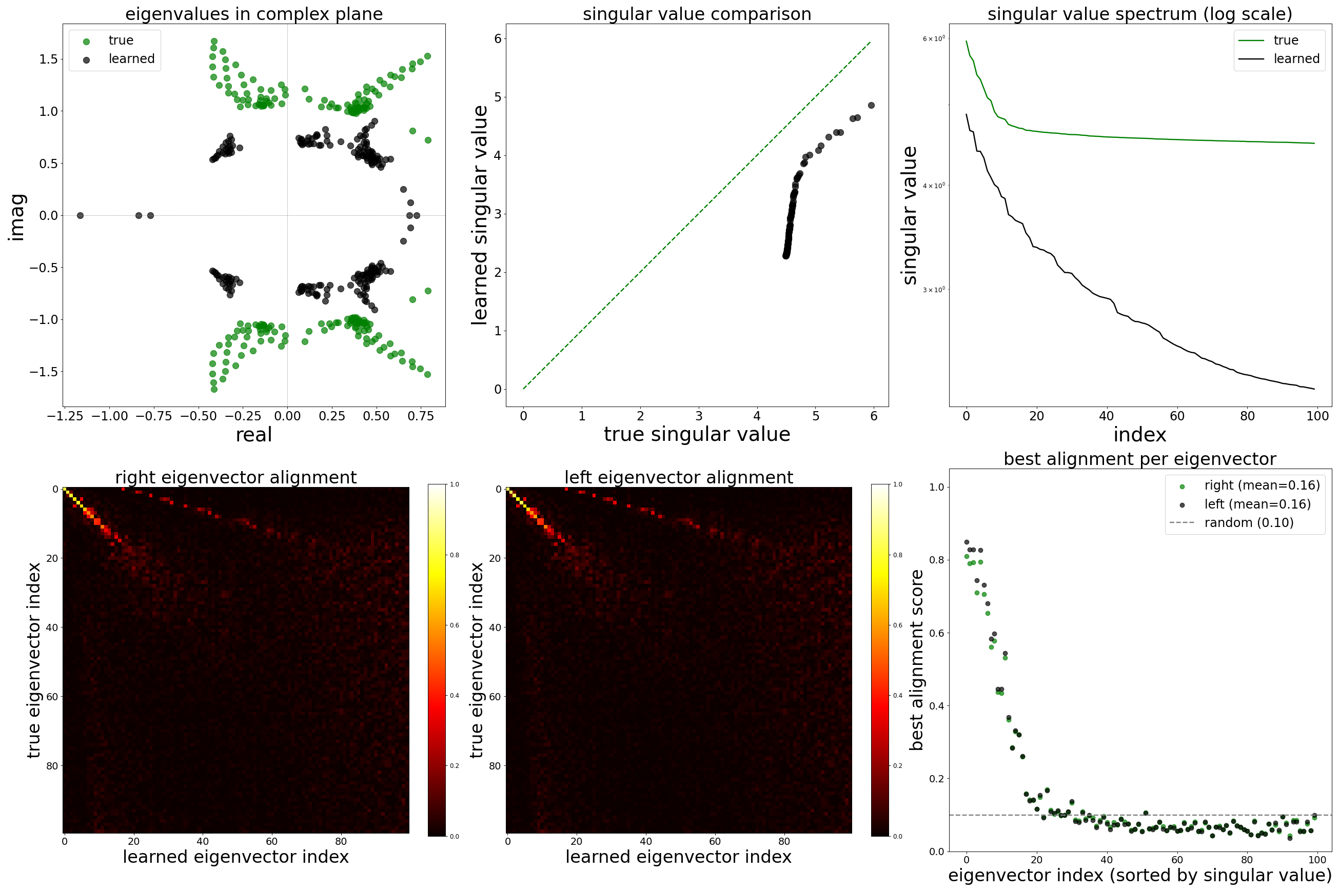
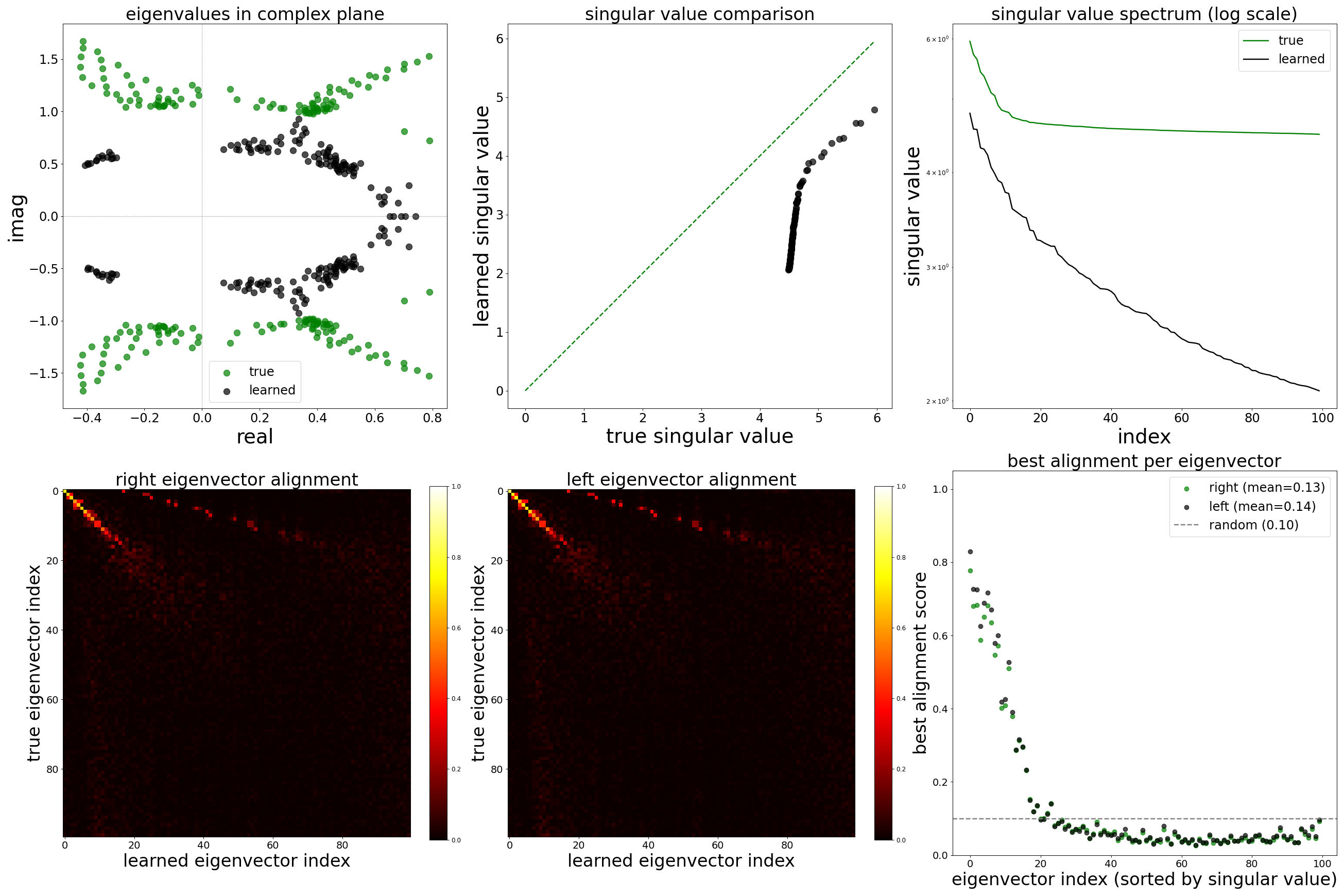
Spectral Analysis
\(\sigma_{\text{meas}} = 0.02\)
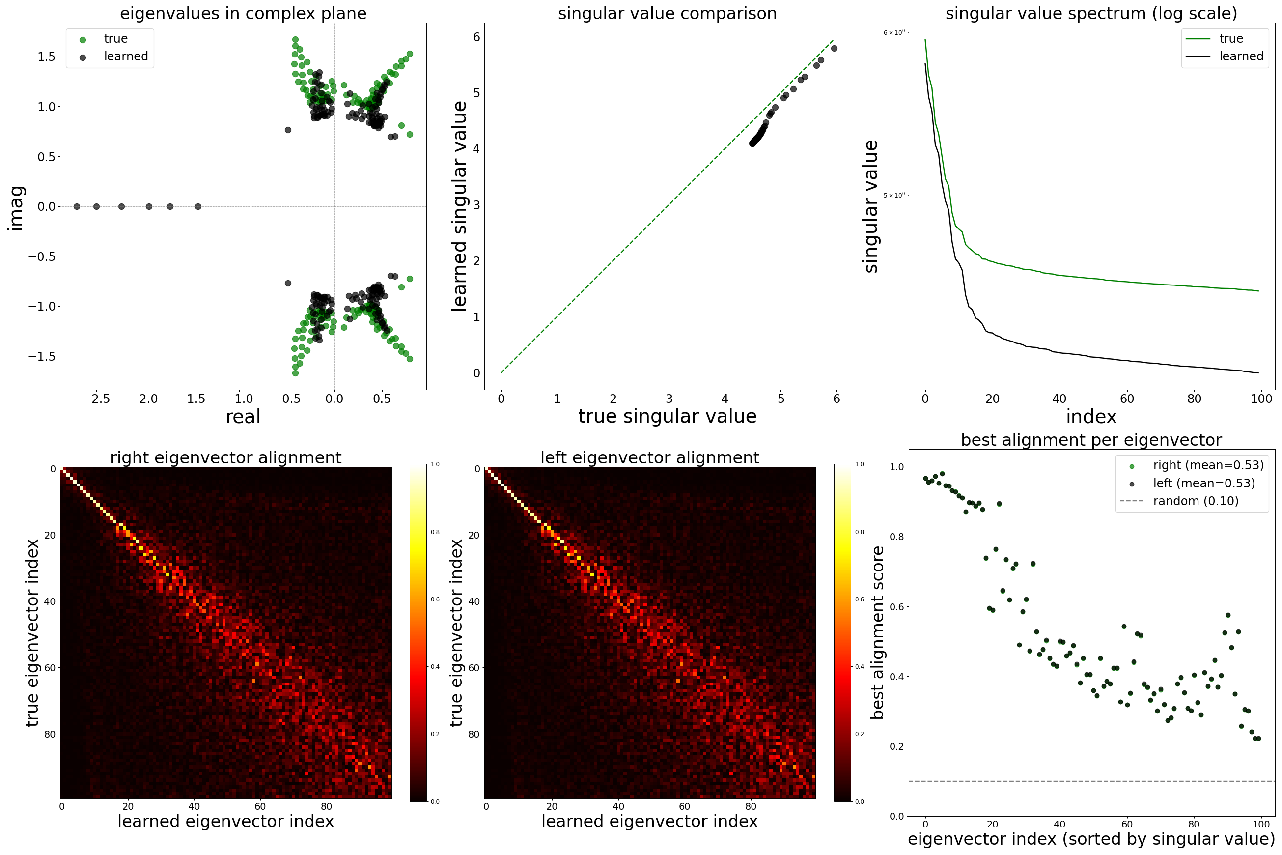
\(\sigma_{\text{meas}} = 0.04\)
\(\sigma_{\text{meas}} = 0.06\)
\(\sigma_{\text{meas}} = 0.08\)
\(\sigma_{\text{meas}} = 0.10\)
References
[1] J. K. Lappalainen et al., “Connectome-constrained networks predict neural activity across the fly visual system,” Nature, 2024. doi:10.1038/s41586-024-07939-3
[2] C. Allier, L. Heinrich, M. Schneider, S. Saalfeld, “Graph neural networks uncover structure and functions underlying the activity of simulated neural assemblies,” arXiv:2602.13325, 2026. doi:10.48550/arXiv.2602.13325