Extract and compare the learned synaptic weights, time constants, resting potentials, neuron-type embeddings, and MLP functions against the ground-truth simulator parameters across noise conditions.
Author
Allier, Lappalainen, Saalfeld
Analysis of Learned Representations
After training (Notebook 01), we analyzed what the GNN had learned about the circuit. For each noise condition we extracted the learned synaptic weights \(\widehat{W}_{ij}\), neural embeddings \(\mathbf{a}_i\), and the two MLP functions (\(f_\theta\) and \(g_\phi\)), and compared them to the ground-truth parameters of the simulator.
The analysis addressed several questions: (1) how accurately did the GNN recover the 434,112 synaptic weights from voltage data alone? (2) did the learned embeddings capture cell-type identity? (3) were the learned functions biologically interpretable? We generated all results plots via data_plot and then display the key results side by side across noise conditions for comparison. Recall that the simulated dynamics include an intrinsic noise term \(\sigma\,\xi_i(t)\) where \(\xi_i(t) \sim \mathcal{N}(0,1)\) (Notebook 00). We compared results at three noise levels: \(\sigma = 0\) (noise-free), \(\sigma = 0.05\) (low noise), and \(\sigma = 0.5\) (high noise).
Configuration
Generate Analysis Plots
For each noise condition, data_plot loads the best model checkpoint and generates the full suite of results visualizations: weight scatter plots (raw and corrected), neural embeddings, MLP function curves, spectral analysis, and UMAP projections.
Code
print()print("="*80)print("ANALYSIS - Generating results plots for all noise conditions")print("="*80)for config_name, label in datasets: config = configs[config_name]print(f"\n--- {label} ---") data_plot( config=config, config_file=config.config_file, epoch_list=['best'], style='color', extended='plots', device=device, )
Connectivity Recovery
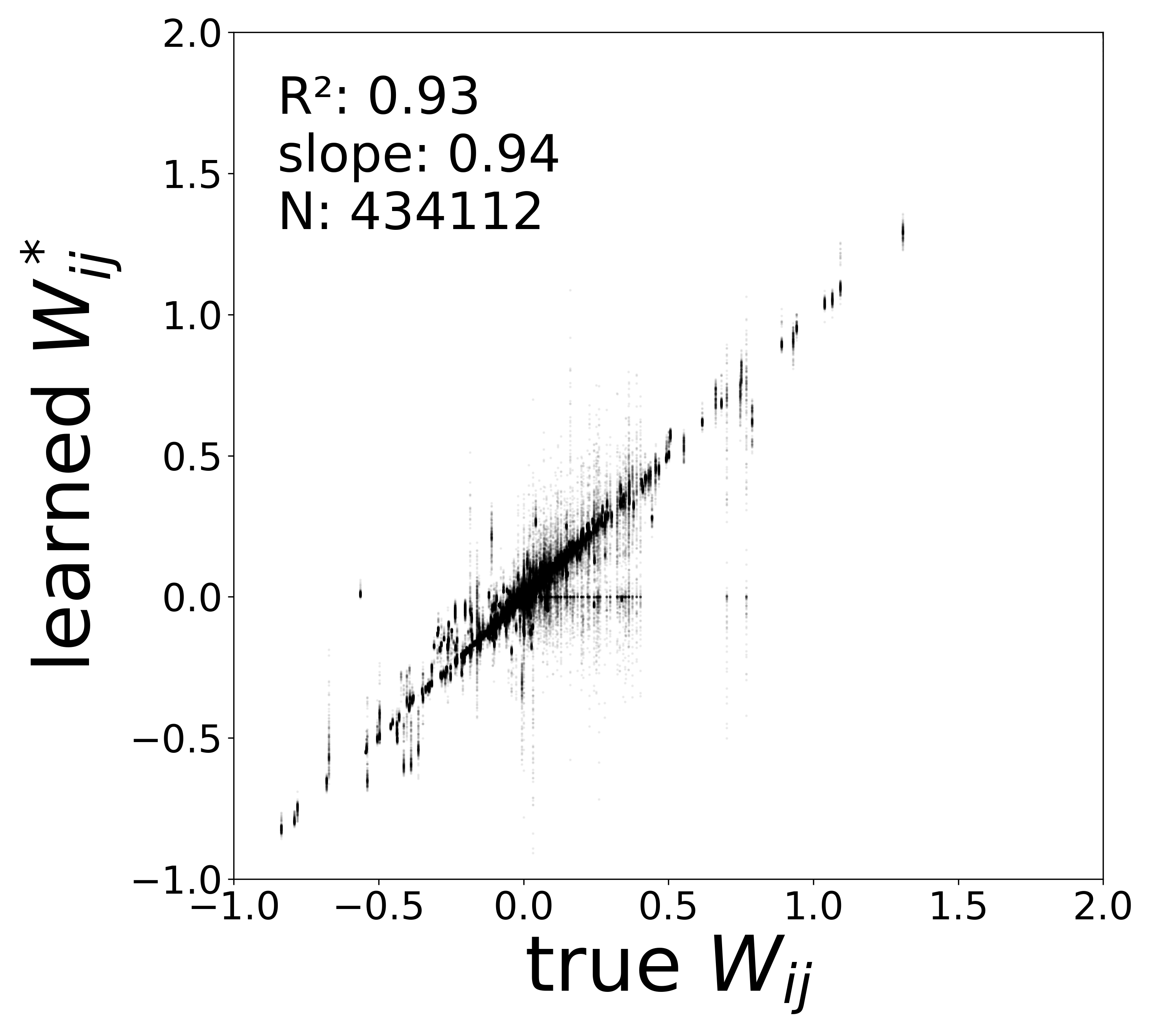
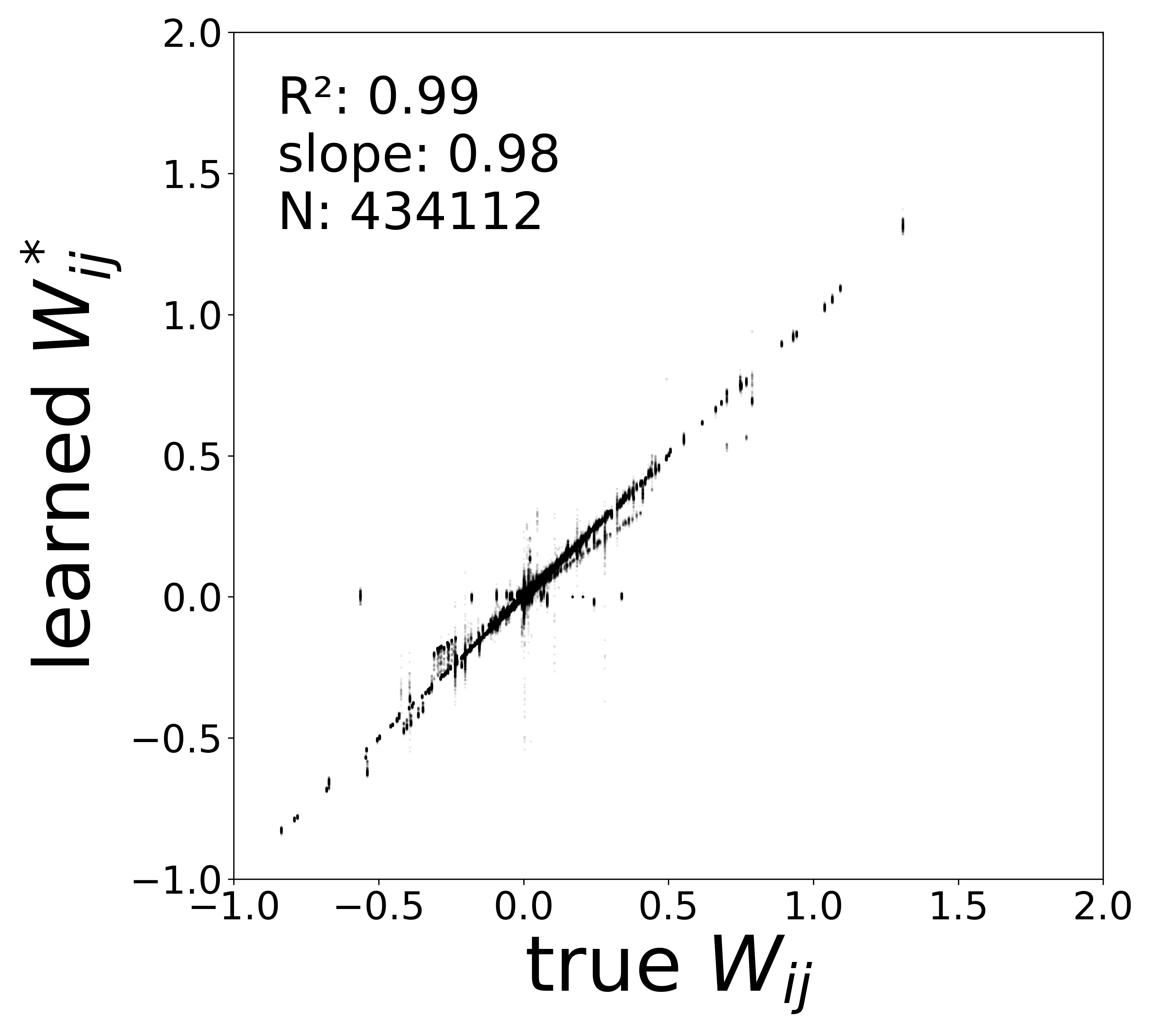
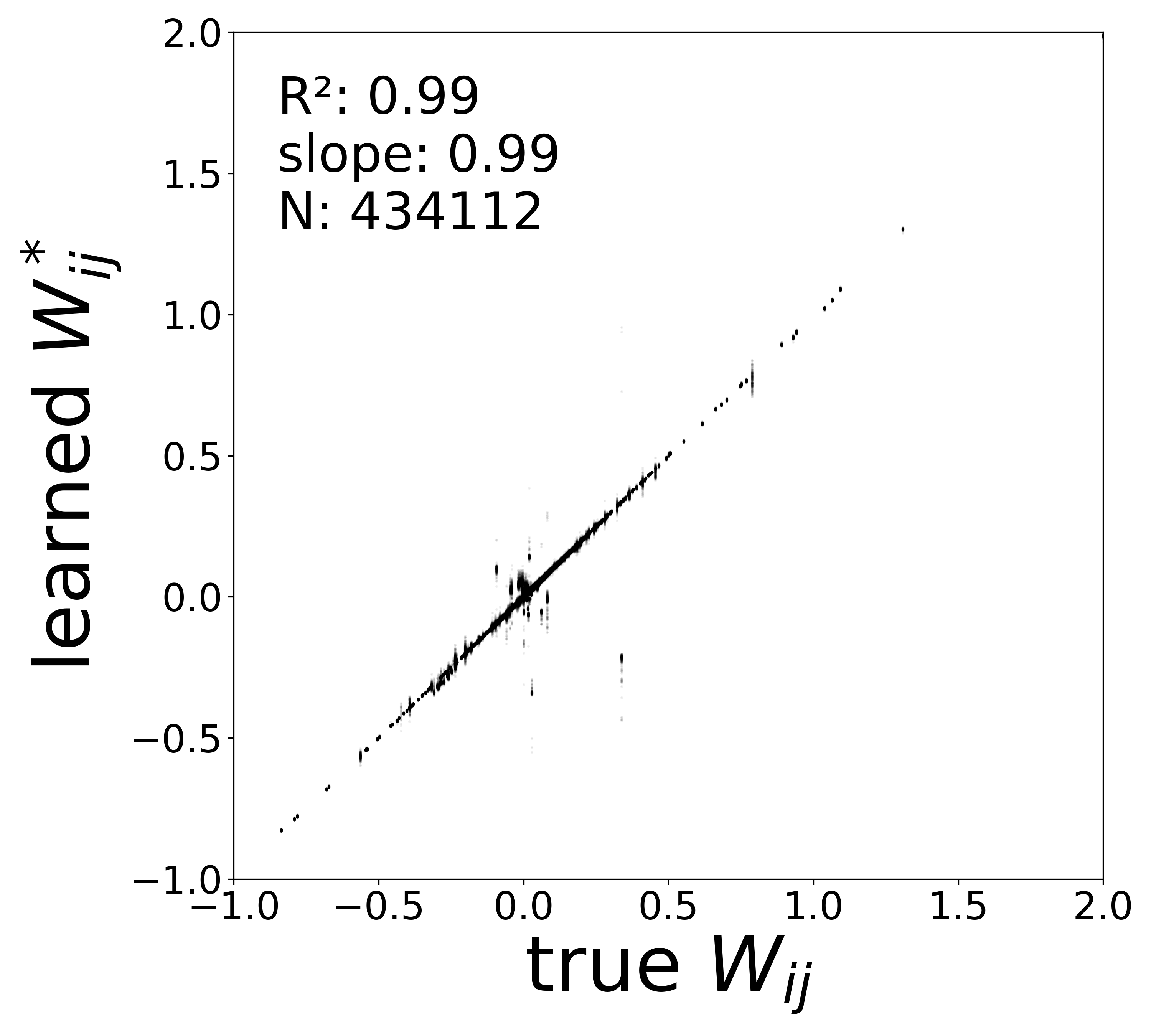
The scatter plots below compare the learned synaptic weights \(\widehat{W}_{ij}\) against the ground-truth connectome weights \(\mathbf{W}_{ij}\) for all 434,112 edges. Because the GNN can absorb arbitrary gain factors into \(f_\theta\) and \(g_\phi\), the raw model parameter \(\widehat{\mathbf{W}}\) differs from the true weights by a per-neuron scaling. The plots show corrected weights that factor out these gains to reveal the true synaptic structure (see below).
Weight–Gain Entanglement. In the GNN forward pass, the message arriving at neuron \(i\) is \(\text{msg}_i = \sum_{j} \widehat{W}_{ij}\,g_\phi(v_j,\mathbf{a}_j)^2\). The model therefore learns the product\(\widehat{W}_{ij} \cdot g_\phi^2\), not \(\widehat{W}_{ij}\) alone: an arbitrary gain absorbed into \(g_\phi\) can be compensated by rescaling \(\widehat{W}_{ij}\), and likewise for the postsynaptic gain of \(f_\theta\). To disentangle the true synaptic weight from these gain factors, we fit a linear model to each function in its activity range (mean \(\pm\) 2 std), extracting per-neuron slopes \(s_g(j)\) from \(g_\phi\) and \(s_f(i)\) from \(f_\theta\), together with \(\partial f_\theta / \partial\text{msg}\) evaluated at typical operating points. The corrected weight is then
which factors out the gain ambiguity and recovers the true synaptic structure, as shown below.
Noise-free (\(\sigma = 0\))
Low noise (\(\sigma = 0.05\))
High noise (\(\sigma = 0.5\))
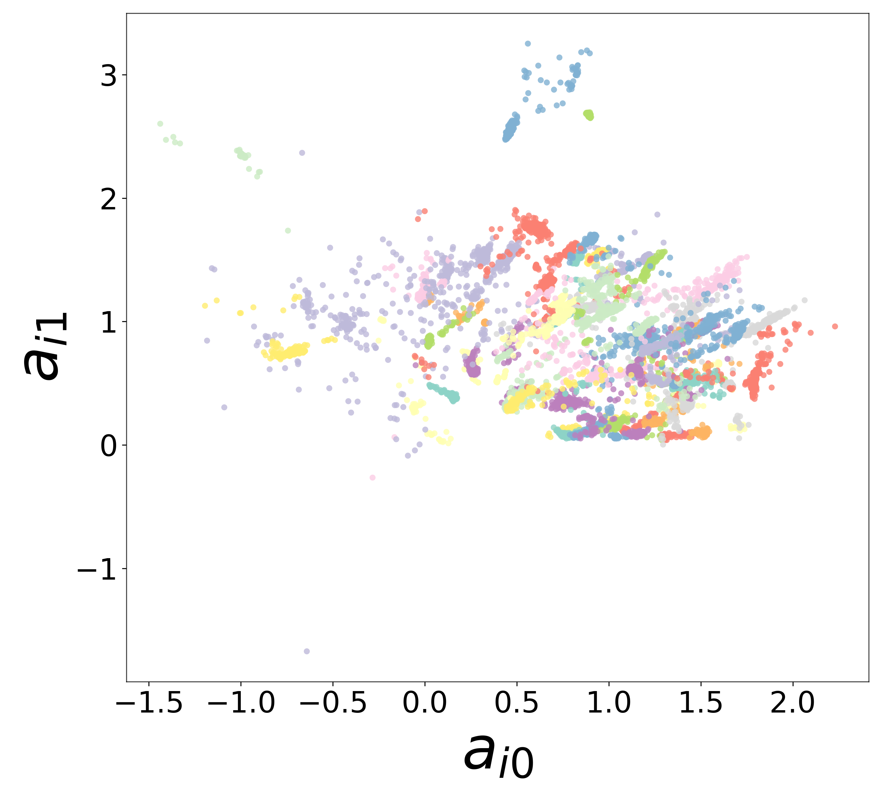
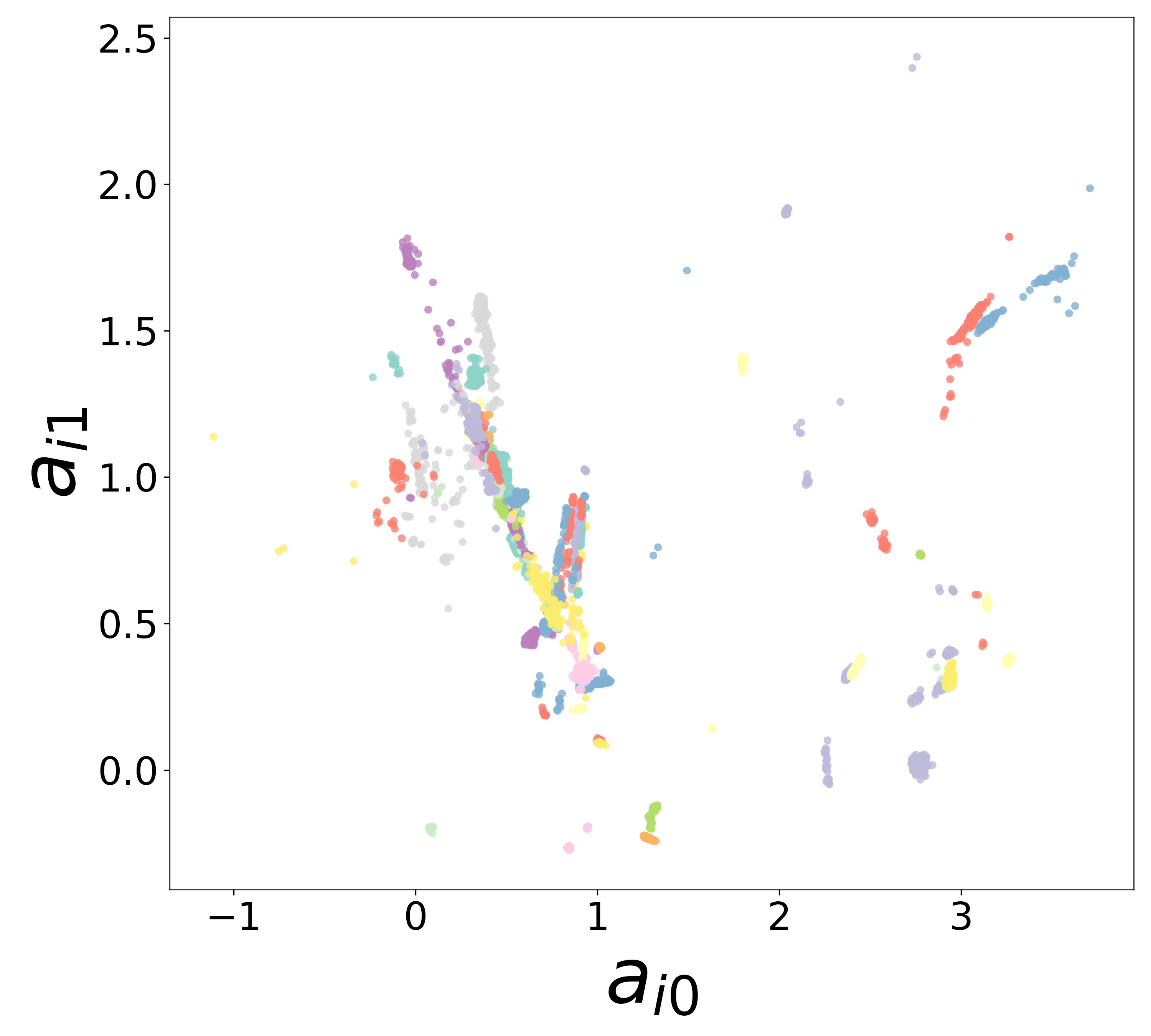
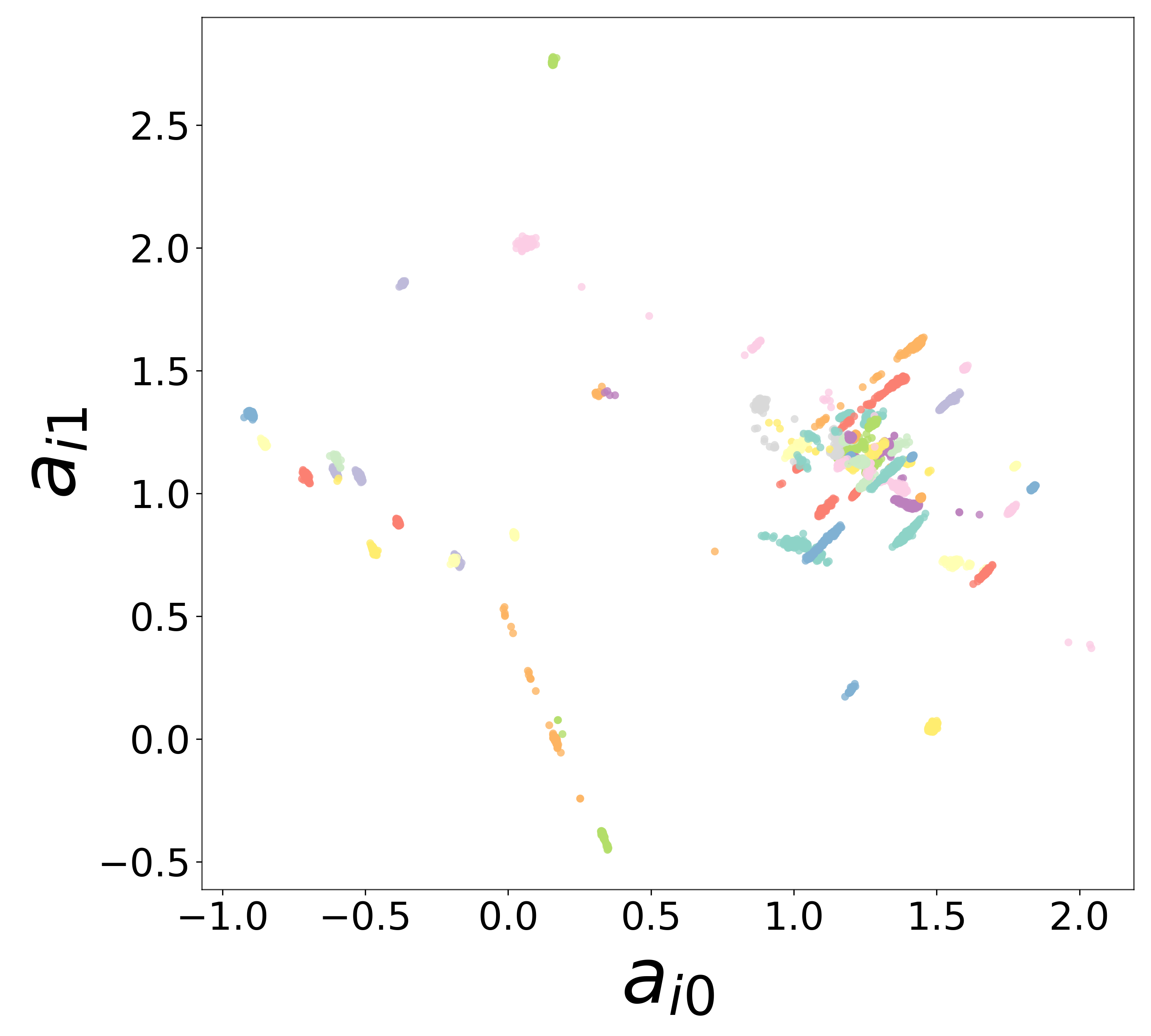
Neural Embeddings
Each neuron \(i\) is assigned a learned embedding vector \(\mathbf{a}_i \in \mathbb{R}^{d_\text{emb}}\) that captures its functional identity. The 2D scatter below shows these embeddings colored by ground-truth cell type. Tight clustering by type indicates that the GNN has discovered cell-type identity from voltage dynamics alone, without any explicit labels.
Noise-free (\(\sigma = 0\))
Low noise (\(\sigma = 0.05\))
High noise (\(\sigma = 0.5\))
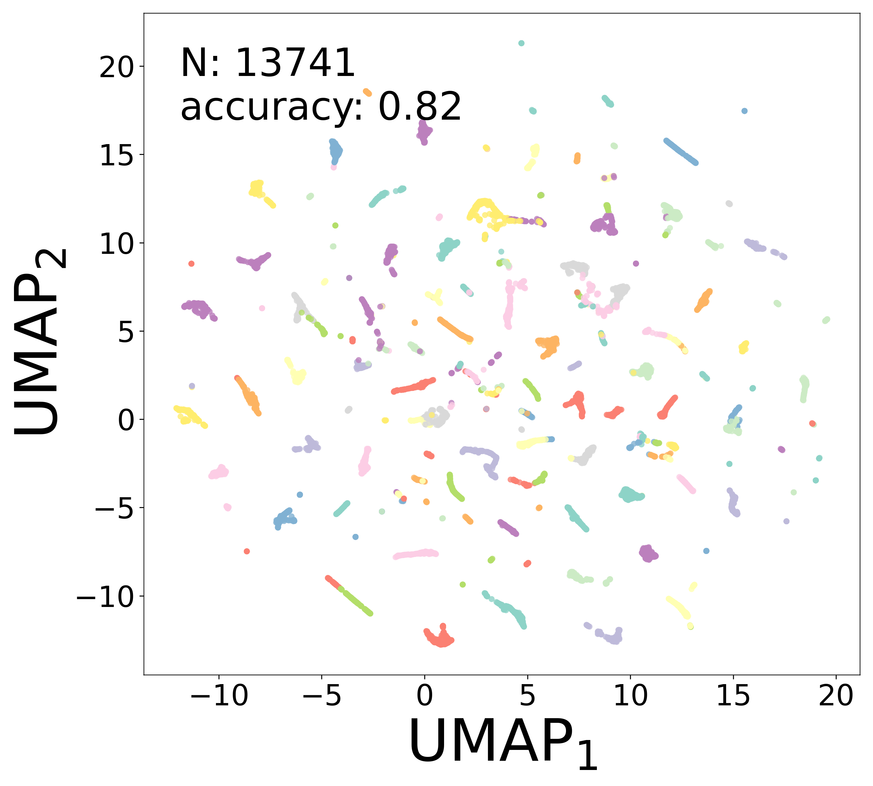
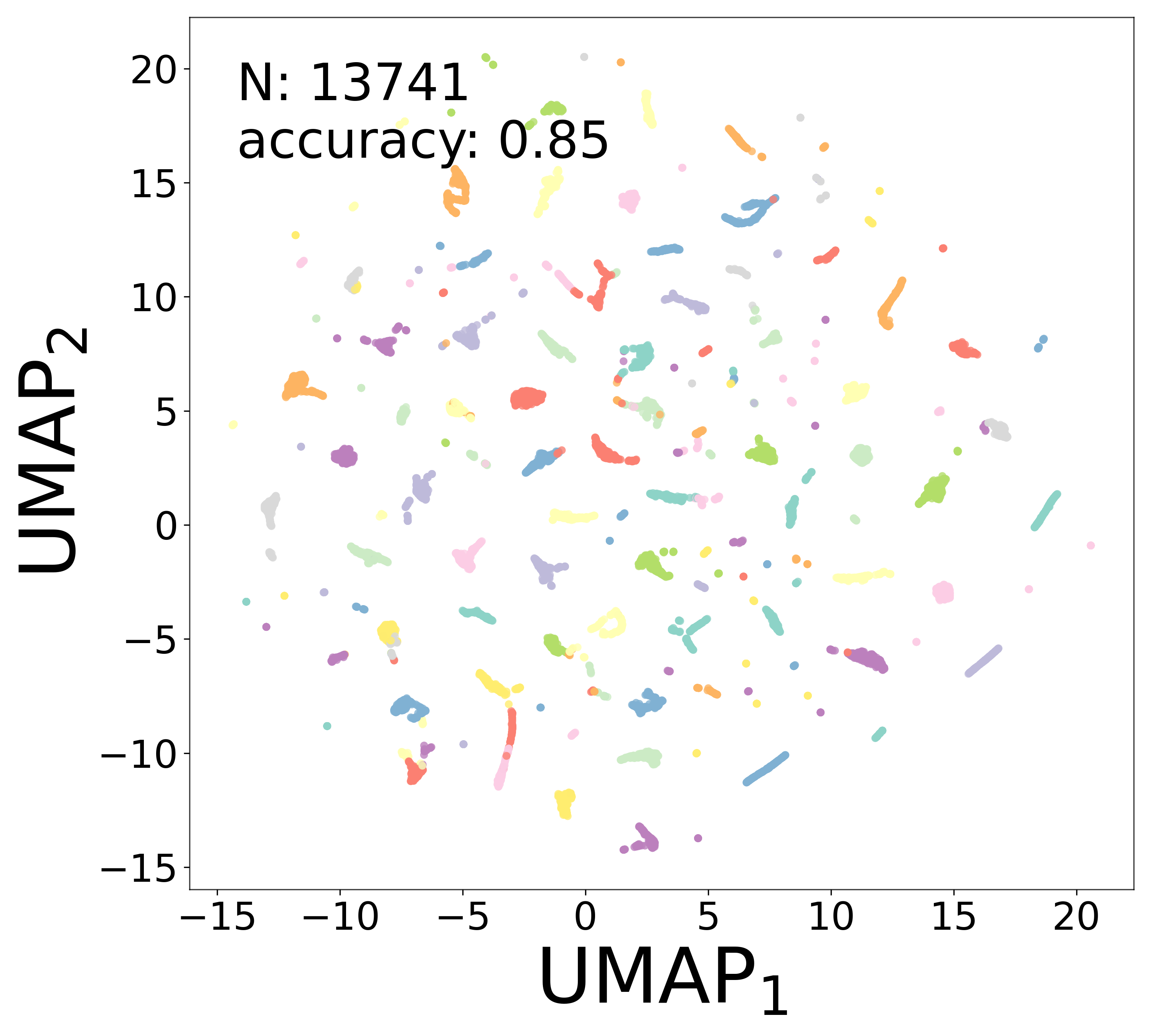
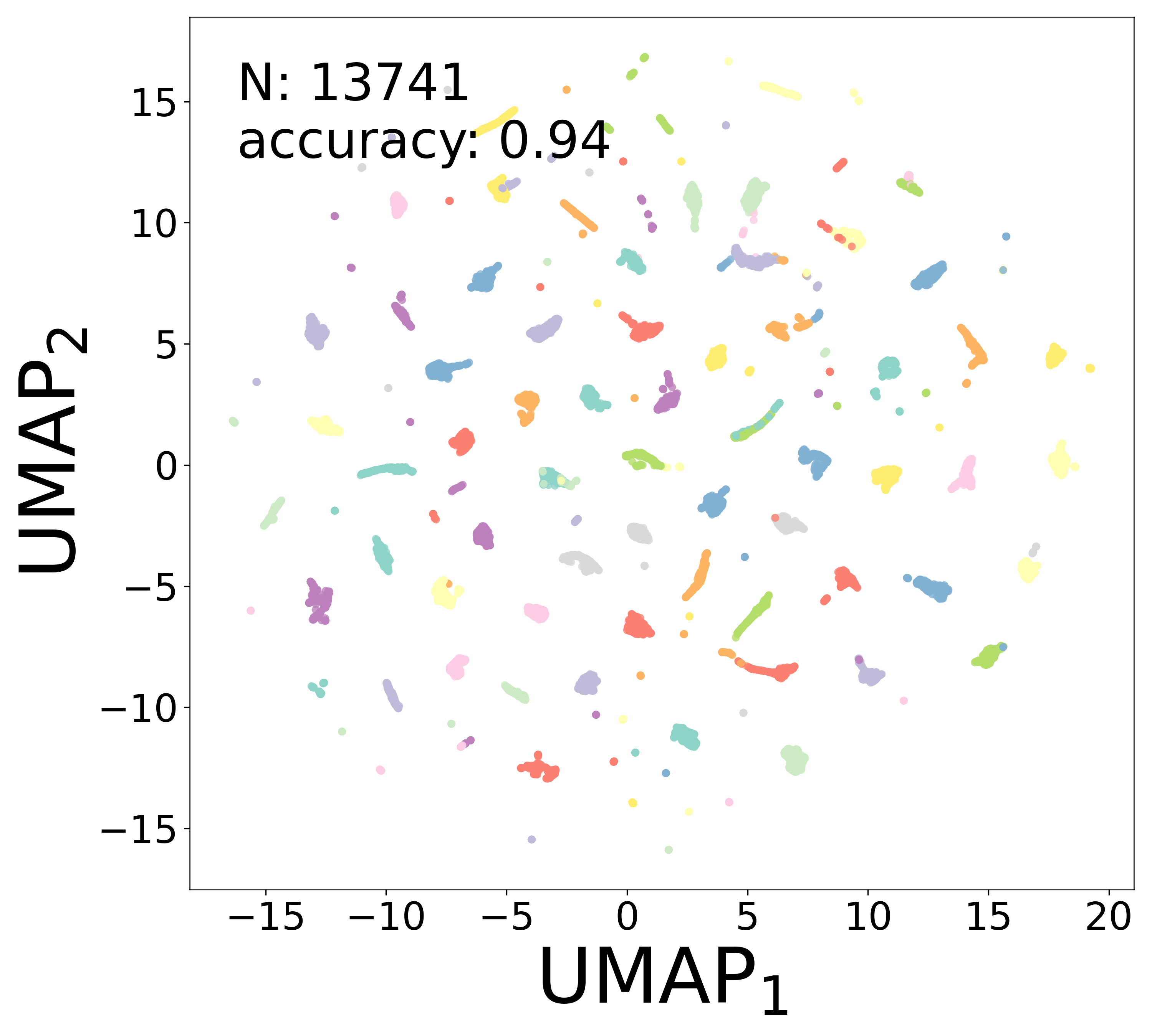
UMAP Projections
To further assess how well the learned representations capture cell-type structure, we apply UMAP [3] to an augmented feature vector that combines the learned embedding \(\mathbf{a}_i\) with the extracted biophysical parameters (\(\tau_i\), \(V_i^{\text{rest}}\)) and connectivity statistics (mean and standard deviation of incoming and outgoing weights). Points are colored by Gaussian mixture model (GMM) cluster labels (\(n_{\text{components}} = 100\)), and the clustering accuracy relative to the ground-truth cell types is reported.
Noise-free (\(\sigma = 0\))
Low noise (\(\sigma = 0.05\))
High noise (\(\sigma = 0.5\))
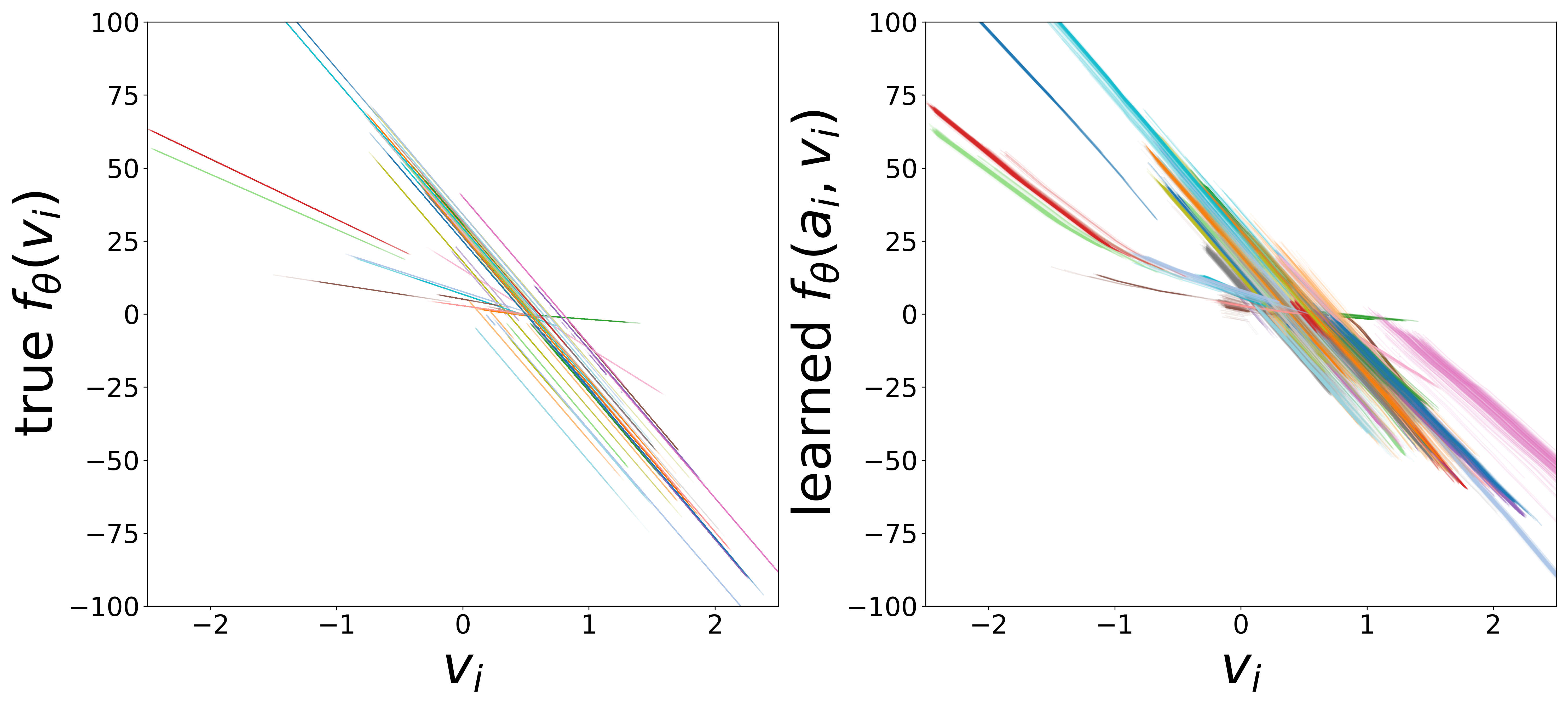
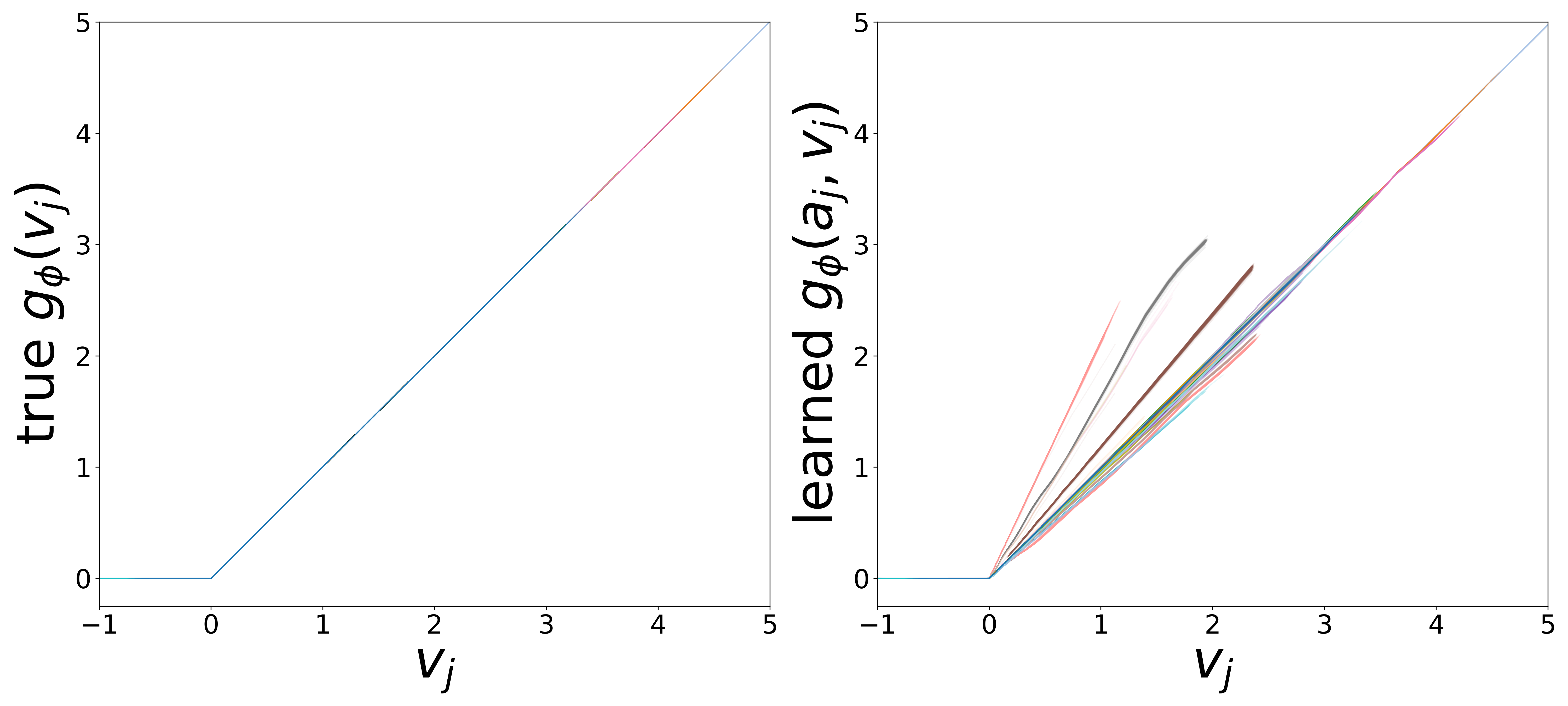
Learned Functions
The GNN uses two MLP functions. The edge message function \(g_\phi\) (MLP\(_1\)) maps presynaptic voltage and embedding to a nonnegative message (via squaring). The monotonicity regularizer (\(\mu_0\)) enforces that \(g_\phi\) increases with voltage, ensuring that stronger presynaptic activity produces larger messages. The neuron update function \(f_\theta\) (MLP\(_0\)) combines postsynaptic voltage, aggregated input, and external stimulus to predict \(\widehat{dv}/dt\).
Each curve corresponds to one of the 65 cell types, colored consistently across plots. The voltage axis is restricted to each neuron type’s activity range (mean \(\pm\) 2 std), where the functions are actually evaluated during inference.
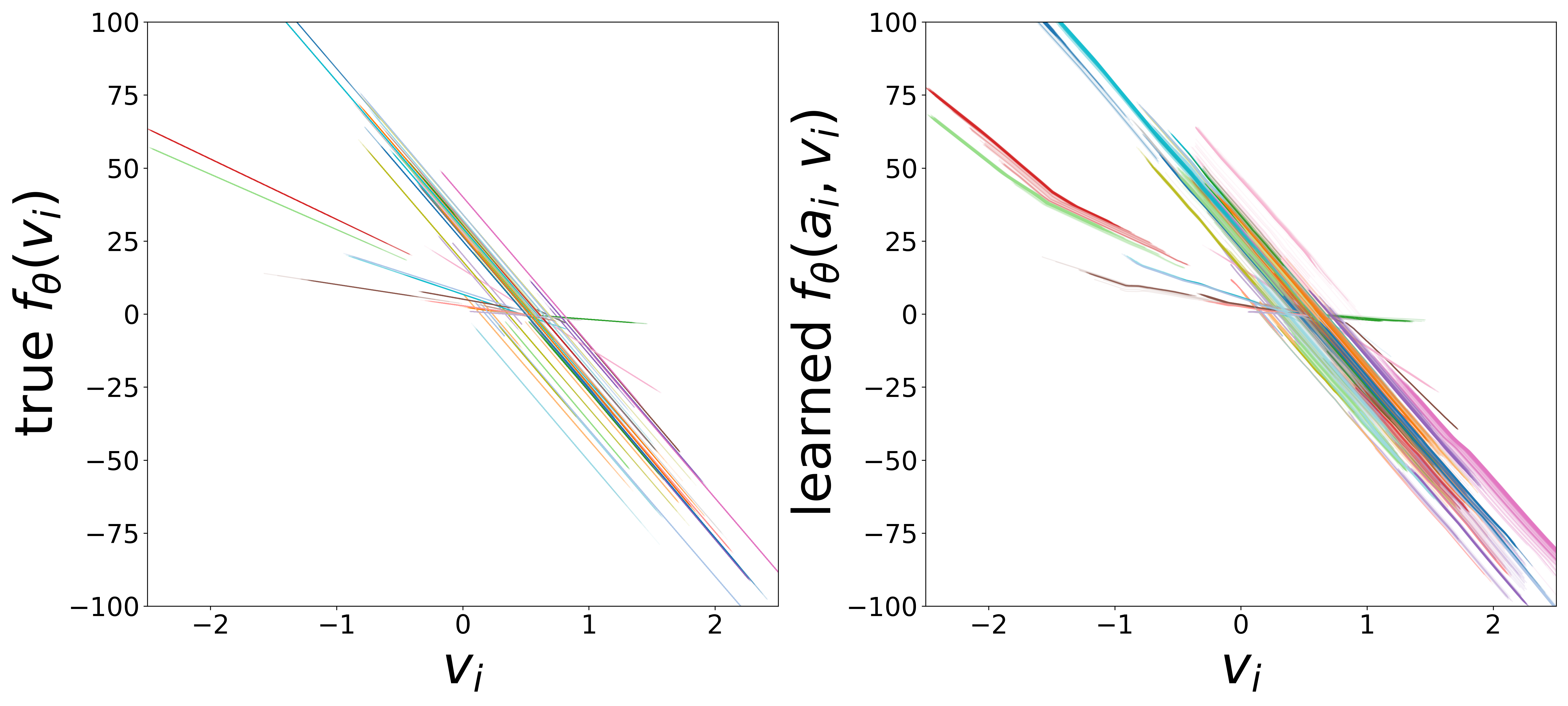
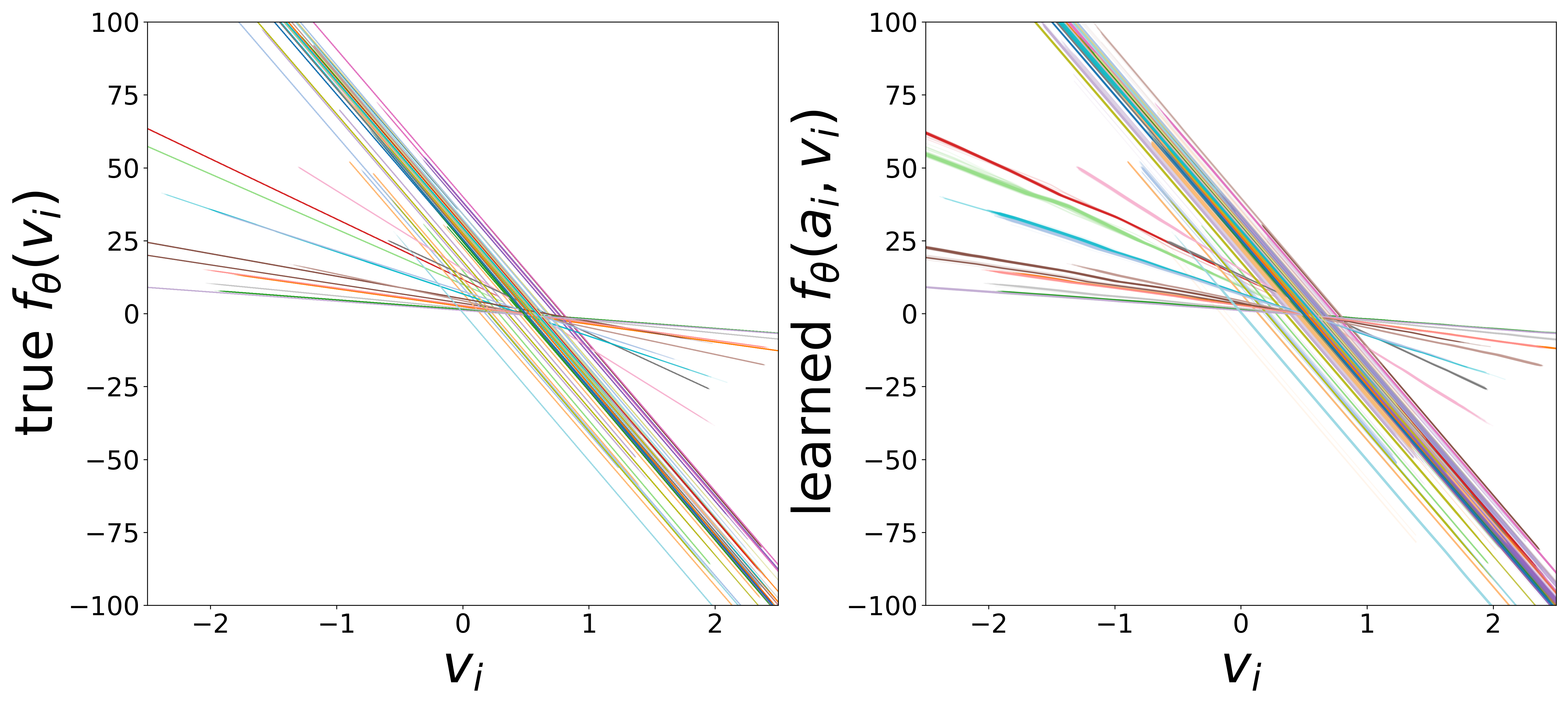
\(f_\theta\) (MLP\(_0\)): Neuron Update Function
Each curve shows \(f_\theta\) restricted to the neuron type’s activity range (mean \(\pm\) 2 std). A linear fit in this domain yields the effective time constant \(\tau_i\) (slope) and resting potential \(V_i^{\text{rest}}\) (zero-crossing), compared to the ground-truth simulator parameters below.
Noise-free (\(\sigma = 0\))
Low noise (\(\sigma = 0.05\))
High noise (\(\sigma = 0.5\))
Biophysical Parameters from \(f_\theta\)
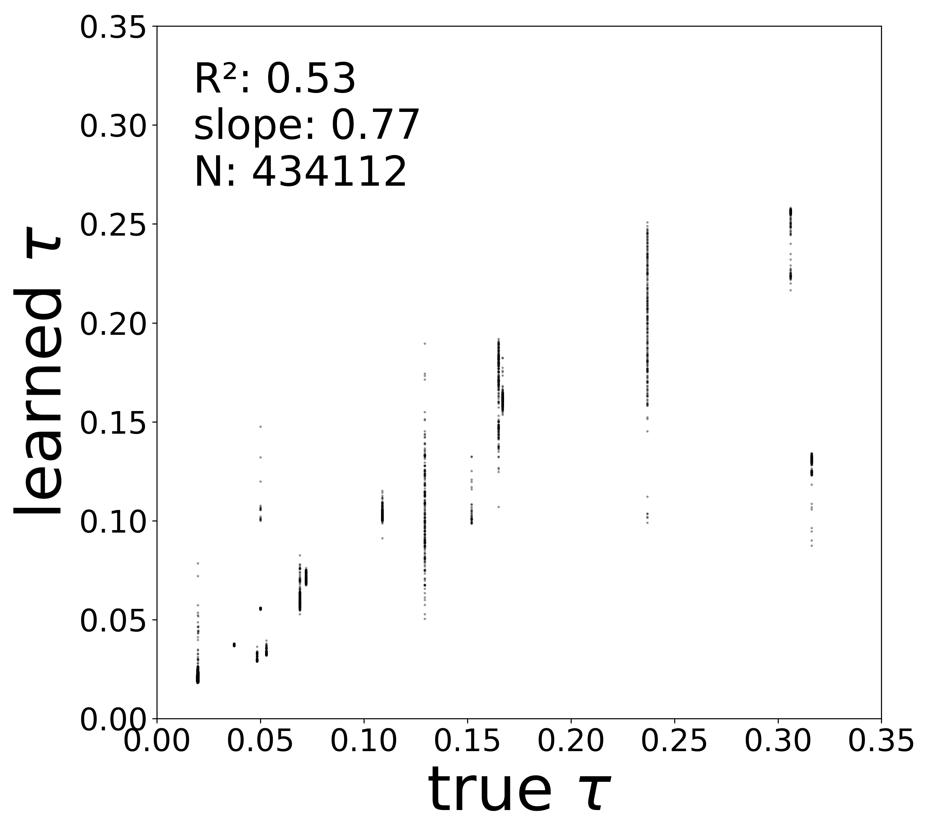
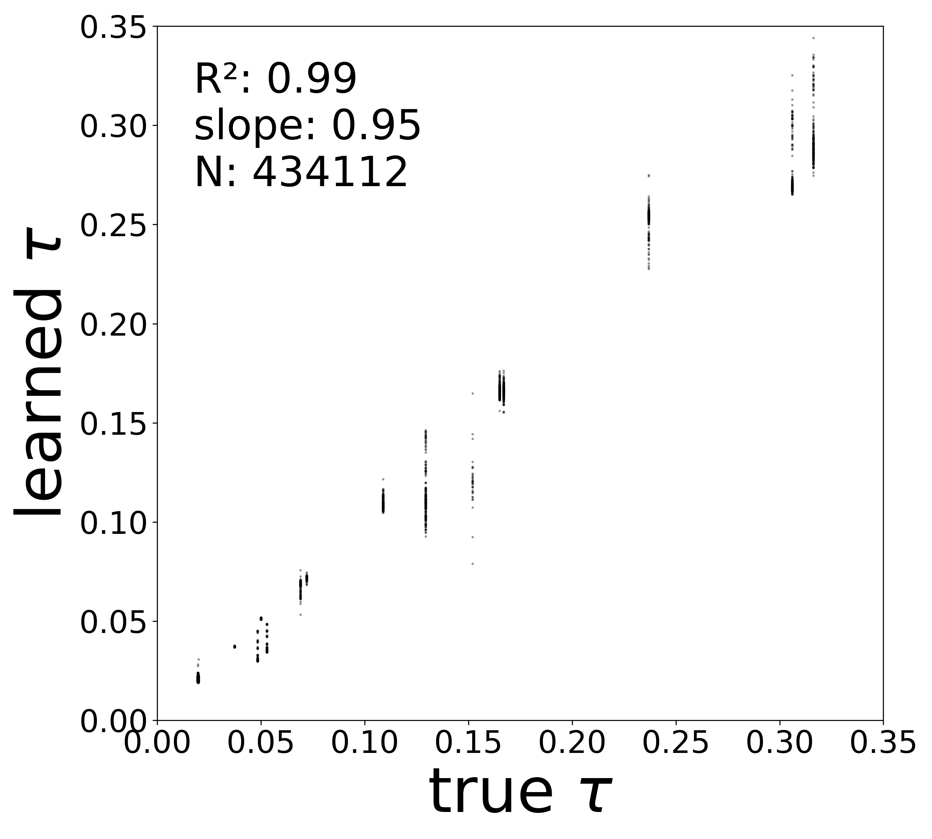
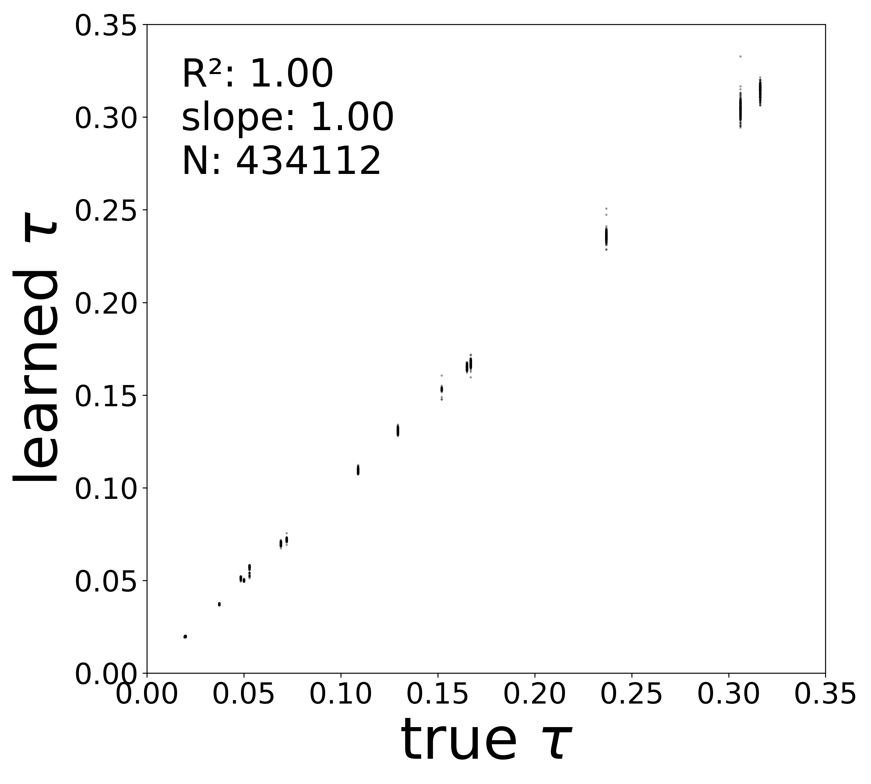
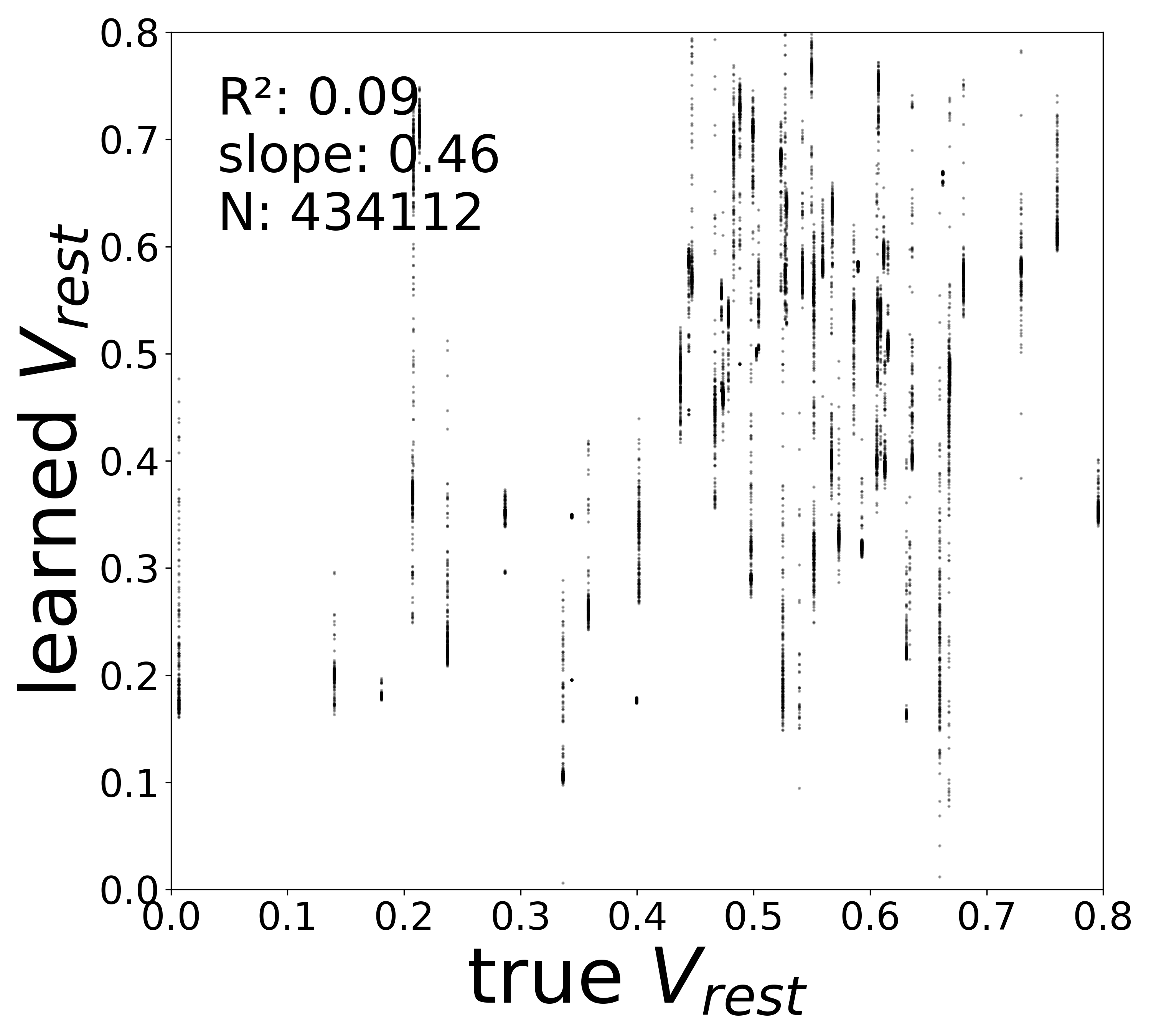
The linear fit to \(f_\theta\) in the natural activity domain directly yields two biophysical parameters for each neuron: the time constant \(\tau_i\) (from the slope) and the resting potential \(V_i^{\text{rest}}\) (from the zero-crossing). The scatter plots below compare these extracted values to the ground-truth simulator parameters.
Time Constants (\(\tau\))
Noise-free (\(\sigma = 0\))
Low noise (\(\sigma = 0.05\))
High noise (\(\sigma = 0.5\))
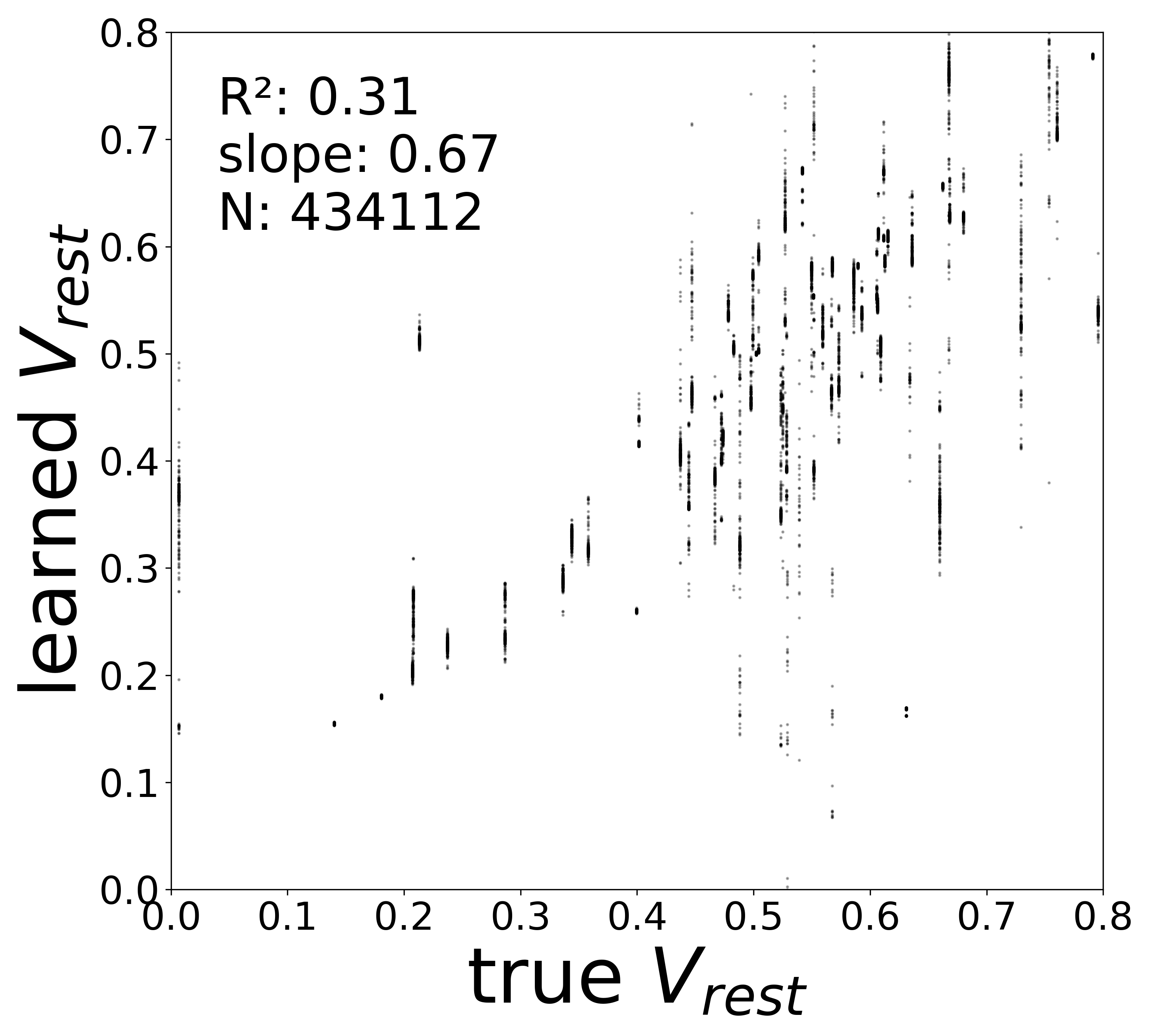
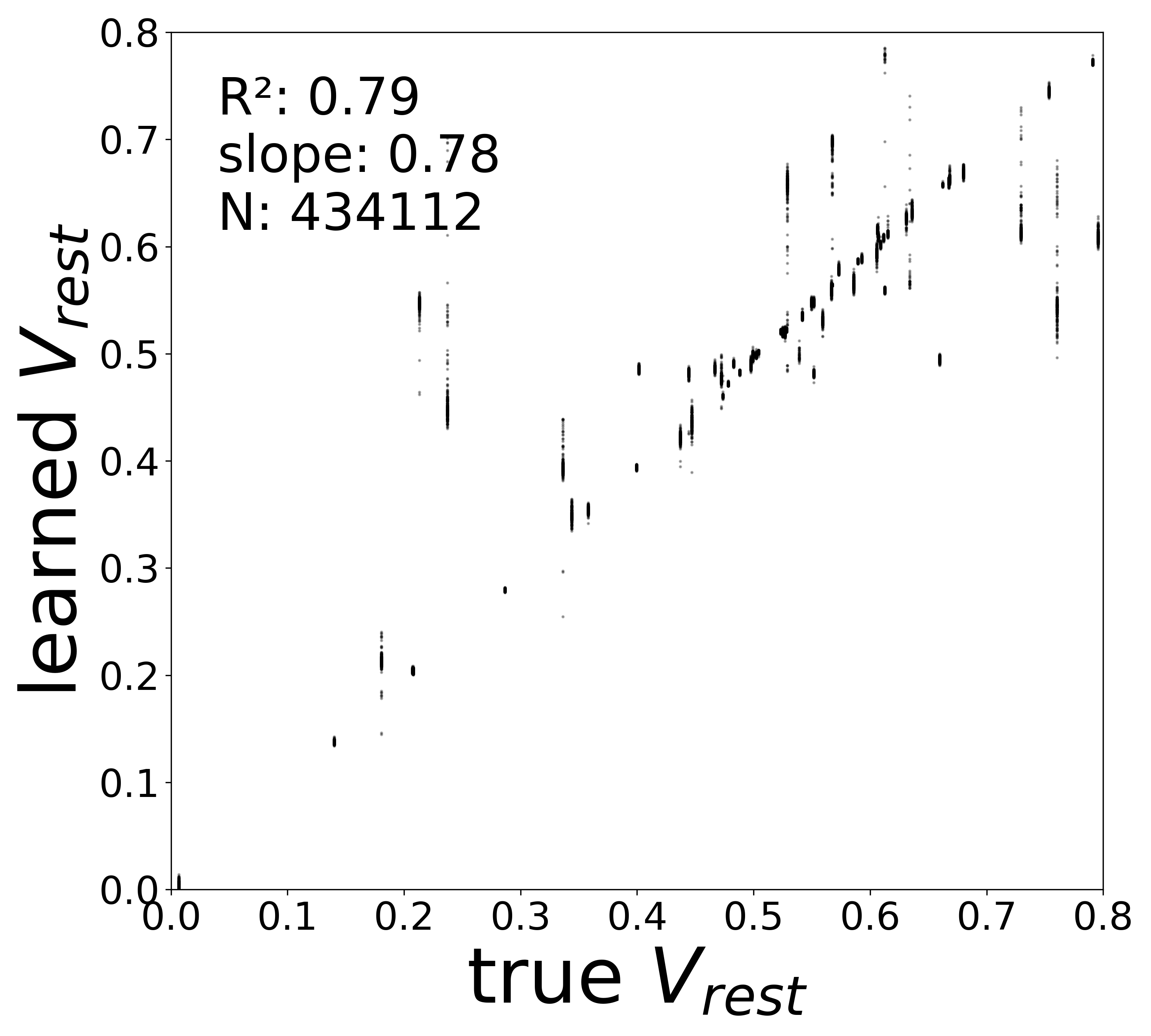
Resting Potentials (\(V^{\text{rest}}\))
Noise-free (\(\sigma = 0\))
Low noise (\(\sigma = 0.05\))
High noise (\(\sigma = 0.5\))
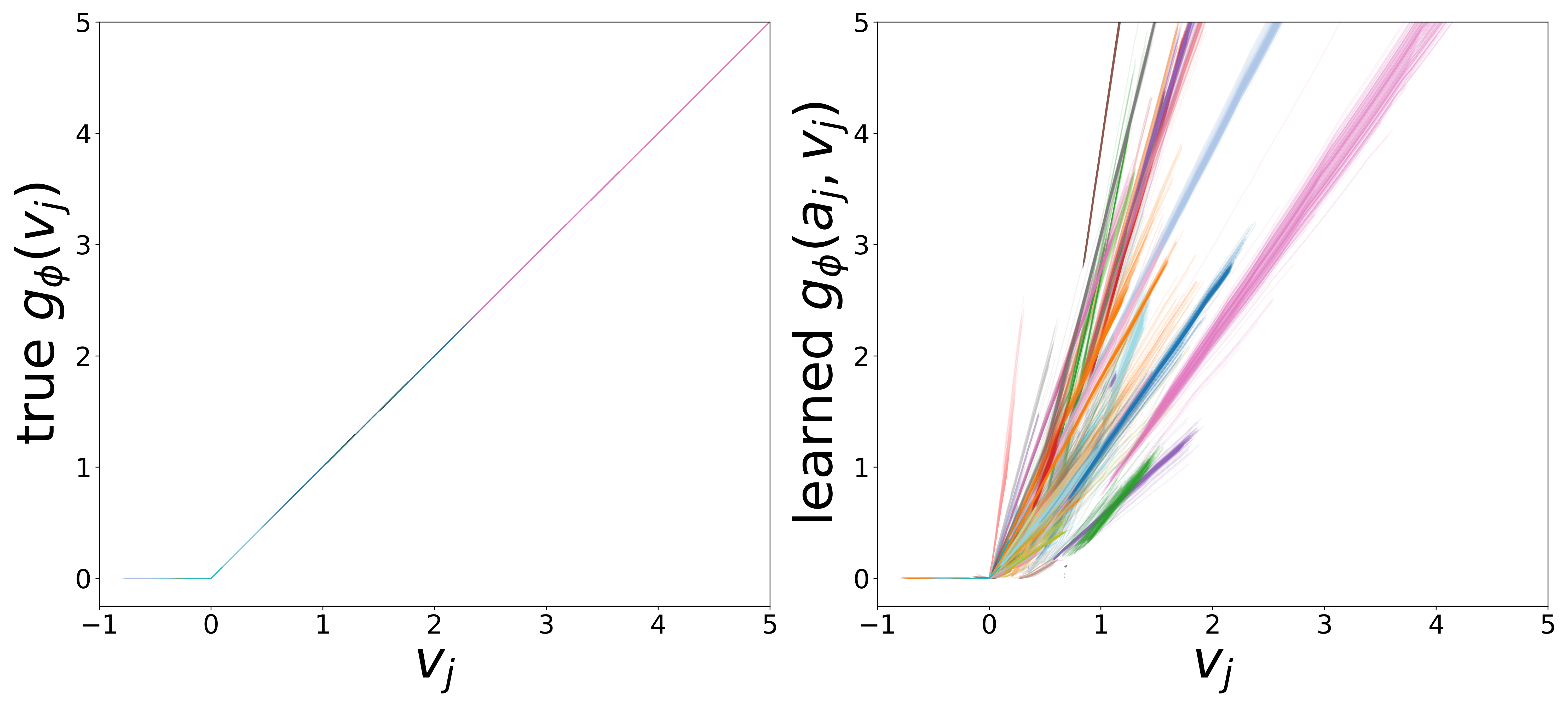
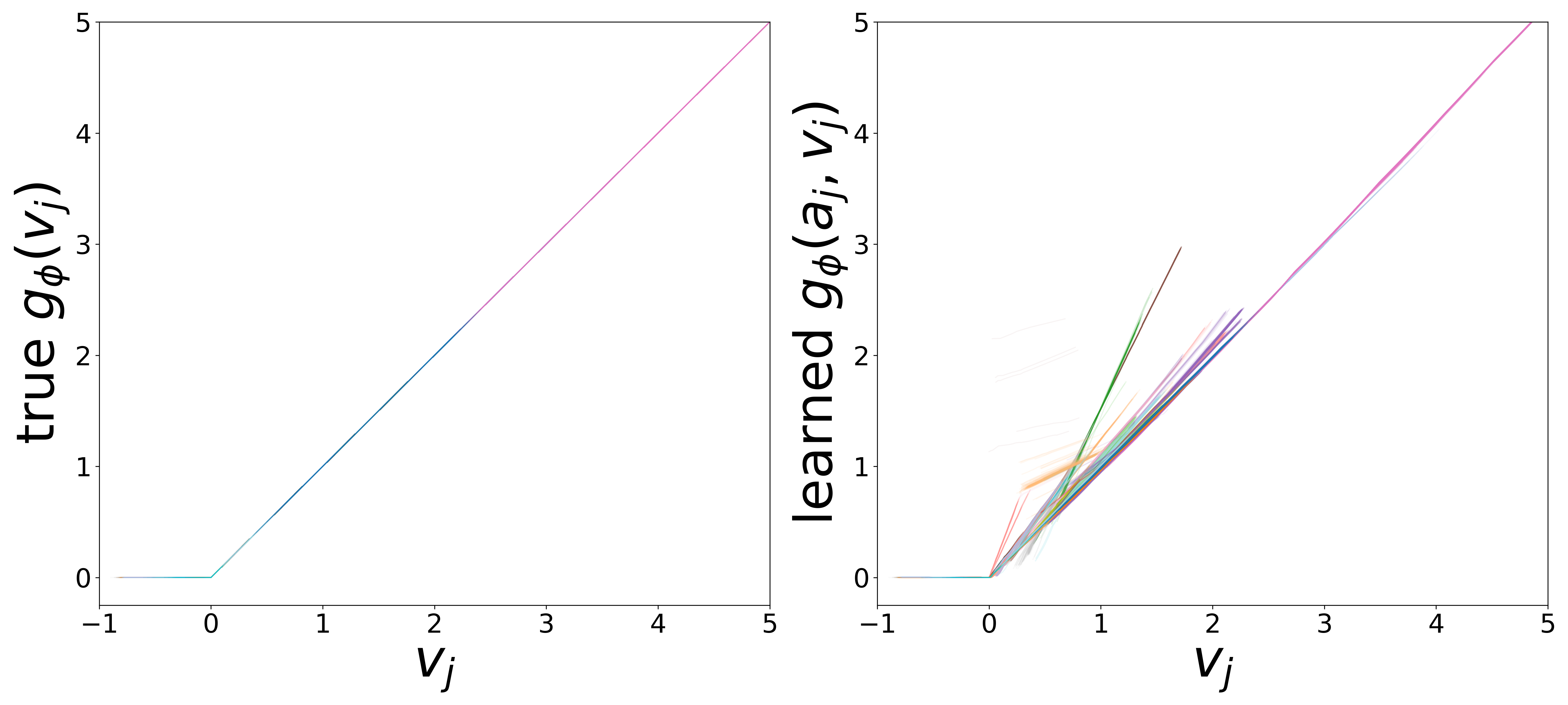
\(g_\phi\) (MLP\(_1\)): Edge Message Function
Each curve shows \(g_\phi\) restricted to the neuron type’s activity range (mean \(\pm\) 2 std). The slopes extracted from the linear fit in this domain are used for the weight correction described above.
Noise-free (\(\sigma = 0\))
Low noise (\(\sigma = 0.05\))
High noise (\(\sigma = 0.5\))
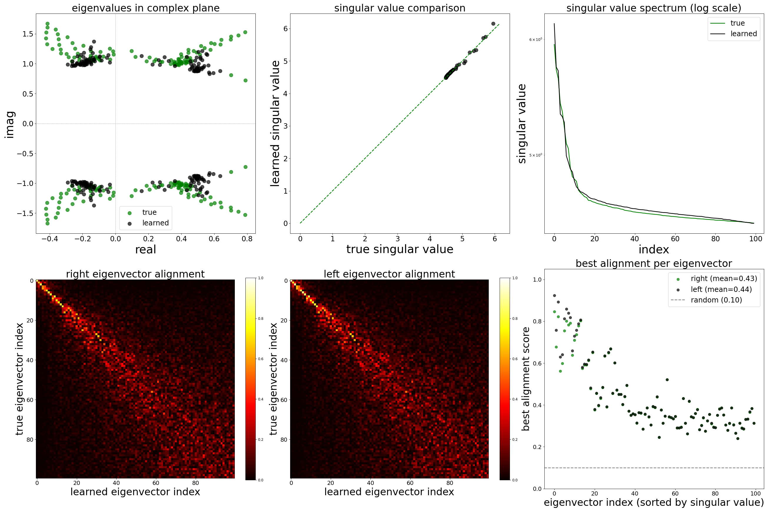
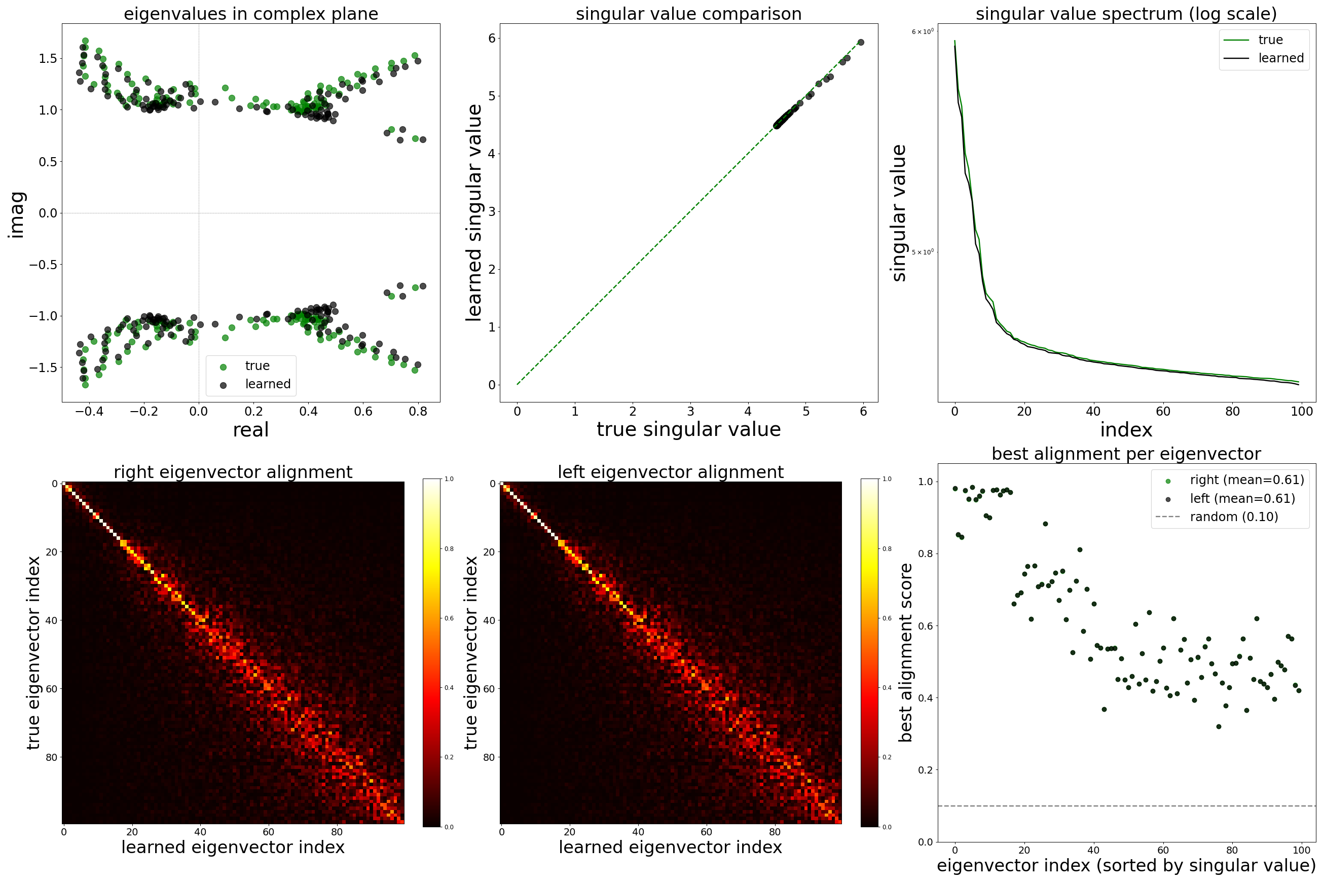
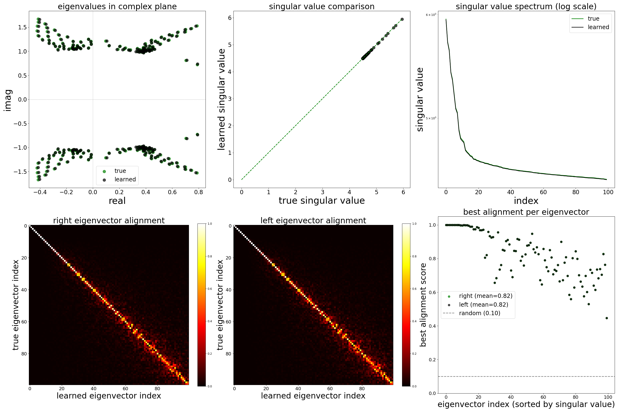
Spectral Analysis
Beyond comparing individual synaptic weights, we ask whether the GNN has recovered the global dynamical structure of the circuit. The weight matrix \(\mathbf{W} \in \mathbb{R}^{N \times N}\) (with \(N{=}13{,}741\) neurons) governs the linear stability and oscillatory modes of the network. Its eigenvalues \(\lambda_k = \text{Re}(\lambda_k) + i\,\text{Im}(\lambda_k)\) determine the time scales and frequencies of intrinsic network modes, while its singular values \(\sigma_k\) capture the gain along principal directions of signal flow.
The \(2 \times 3\) figure below compares the spectral properties of the ground-truth and learned (corrected) weight matrices:
Top row.Eigenvalues and singular values. (Left) The 200 largest-magnitude eigenvalues plotted in the complex plane; overlap between green (true) and black (learned) clouds indicates that the GNN preserves the circuit’s oscillatory and decay modes. (Center) A scatter of matched singular values; black points near the diagonal mean the learned matrix preserves the gain spectrum. (Right) The singular value spectrum on a log scale; parallel decay curves confirm that the rank structure and effective dimensionality of the connectivity are faithfully reproduced.
Bottom row.Singular vector alignment. (Left and center) Alignment matrices between the top 100 right and left singular vectors of the true and learned matrices. A strong diagonal indicates one-to-one correspondence between the principal connectivity modes. Off-diagonal mass would signal that the learned matrix mixes true modes. (Right) The best alignment score per singular vector. Values near 1.0 mean the corresponding mode is recovered almost exactly; the gray dashed line marks the expected alignment for random vectors.
Noise-free (\(\sigma = 0\))
Low noise (\(\sigma = 0.05\))
High noise (\(\sigma = 0.5\))
Summary
The table below summarizes the key quantitative metrics across the three noise conditions. Weight correlation (\(R^2\)) is reported for the corrected weights. These metrics are extracted from the results.log files generated by data_plot.
Metric
Noise-free
Noise 0.05
Noise 0.5
\(W\) corrected \(R^2\)
0.9263
0.9852
0.9898
\(W\) corrected slope
0.9415
0.9830
0.9941
\(\tau\)\(R^2\)
0.5277
0.9888
0.9997
\(V^{\text{rest}}\)\(R^2\)
0.0884
0.3104
0.7892
References
[1] J. K. Lappalainen et al., “Connectome-constrained networks predict neural activity across the fly visual system,” Nature, 2024. doi:10.1038/s41586-024-07939-3
[3] L. McInnes, J. Healy, and J. Melville, “UMAP: Uniform Manifold Approximation and Projection for Dimension Reduction,” 2018. doi:10.48550/arXiv.1802.03426