Data Generation: Drosophila Visual System

Simulate the Drosophila visual system with 13,741 neurons across 65 cell types at three intrinsic noise levels (\(\sigma = 0\), \(0.05\), \(0.5\)) and generate voltage traces for GNN training and testing.

Simulation

We simulated neural activity in the Drosophila visual system using flyvis’ pretrained models [1]. The recurrent neural network contains 13,741 neurons from 65 cell types and 434,122 synaptic connections, corresponding to real neurons and their synapses. We restricted the original 721 retinotopic columns to the central subset of 217. Each neuron is modeled as a non-spiking compartment governed by

\[\tau_i\frac{dv_i(t)}{dt} = -v_i(t) + V_i^{\text{rest}} + \sum_{j\in\mathcal{N}_i} \mathbf{W}_{ij}\,\text{ReLU}\!\big(v_j(t)\big) + I_i(t) + \sigma\,\xi_i(t),\]

where \(\tau_i\) and \(V_i^{\text{rest}}\) are cell-type parameters, \(\mathbf{W}_{ij}\) is the connectome-constrained synaptic weight, \(I_i(t)\) the visual input, and \(\xi_i(t) \sim \mathcal{N}(0,1)\) is independent Gaussian noise scaled by \(\sigma\). The noise term \(\sigma\,\xi_i(t)\) models intrinsic stochasticity in the membrane dynamics (e.g. channel noise, synaptic variability).

Unlike measurement noise added post hoc, this intrinsic noise alters the dynamical trajectory of \(v_i(t)\) and couples through the connectivity matrix \(\mathbf{W}\). As a dynamical perturbation, it widens the distribution of visited voltages and propagates through synaptic connections, enriching the training signal.

We generated data at three noise levels \(\sigma\):

Dataset	\(\sigma\)	Description
flyvis_noise_free	0.0	Deterministic (no intrinsic noise)
flyvis_noise_005	0.05	Low intrinsic noise
flyvis_noise_05	0.5	High intrinsic noise

Visual Stimulus

The visual input \(I_i(t)\) is derived from the DAVIS dataset [2, 3], a collection of natural video sequences at 480p resolution originally developed for optical flow and video segmentation benchmarks. Each RGB frame is center-cropped to 60% of its spatial extent, converted to grayscale luminance, and resampled onto the hexagonal photoreceptor lattice of 217 columns via a Gaussian box-eye filter (extent 8, kernel size 13). Each column feeds 8 photoreceptor types (R1–R8), giving 1,736 input neurons. Videos longer than 80 frames are split into 50-frame chunks; temporal interpolation resamples each chunk to match the simulation time step \(\Delta t = 0.02\).

The full set of sequences is augmented with horizontal and vertical flips and four rotations (0°, 90°, 180°, 270°) of the hexagonal array. All augmentations of the same base video are kept together and the dataset is split 80/20 at the base-video level to prevent data leakage between training and testing. The sequences within each split are shuffled (seed 42) and concatenated into a continuous stimulus stream.

print()
print("=" * 80)
print("GENERATE - Simulating fly visual system at three noise levels")
print("=" * 80)

for config_name, label in datasets:
    config = configs[config_name]
    graphs_dir = graphs_dirs[config_name]
    print()
    print(f"--- {label} (noise_model_level={config.simulation.noise_model_level}) ---")

    data_exists = os.path.isdir(f'{graphs_dir}/x_list_train') or os.path.isdir(f'{graphs_dir}/x_list_0')
    if data_exists:
        print(f"  data already exists at {graphs_dir}/")
        print("  skipping simulation...")
    else:
        print(f"  simulating {config.simulation.n_neurons} neurons, {config.simulation.n_neuron_types} types")
        print(f"  generating {config.simulation.n_frames} time frames")
        print(f"  visual input: {config.simulation.visual_input_type}")
        print(f"  output: {graphs_dir}/")
        print()
        data_generate(
            config,
            device=device,
            visualize=True,
            run_vizualized=0,
            style="color",
            alpha=1,
            erase=False,
            save=True,
            step=100,
        )

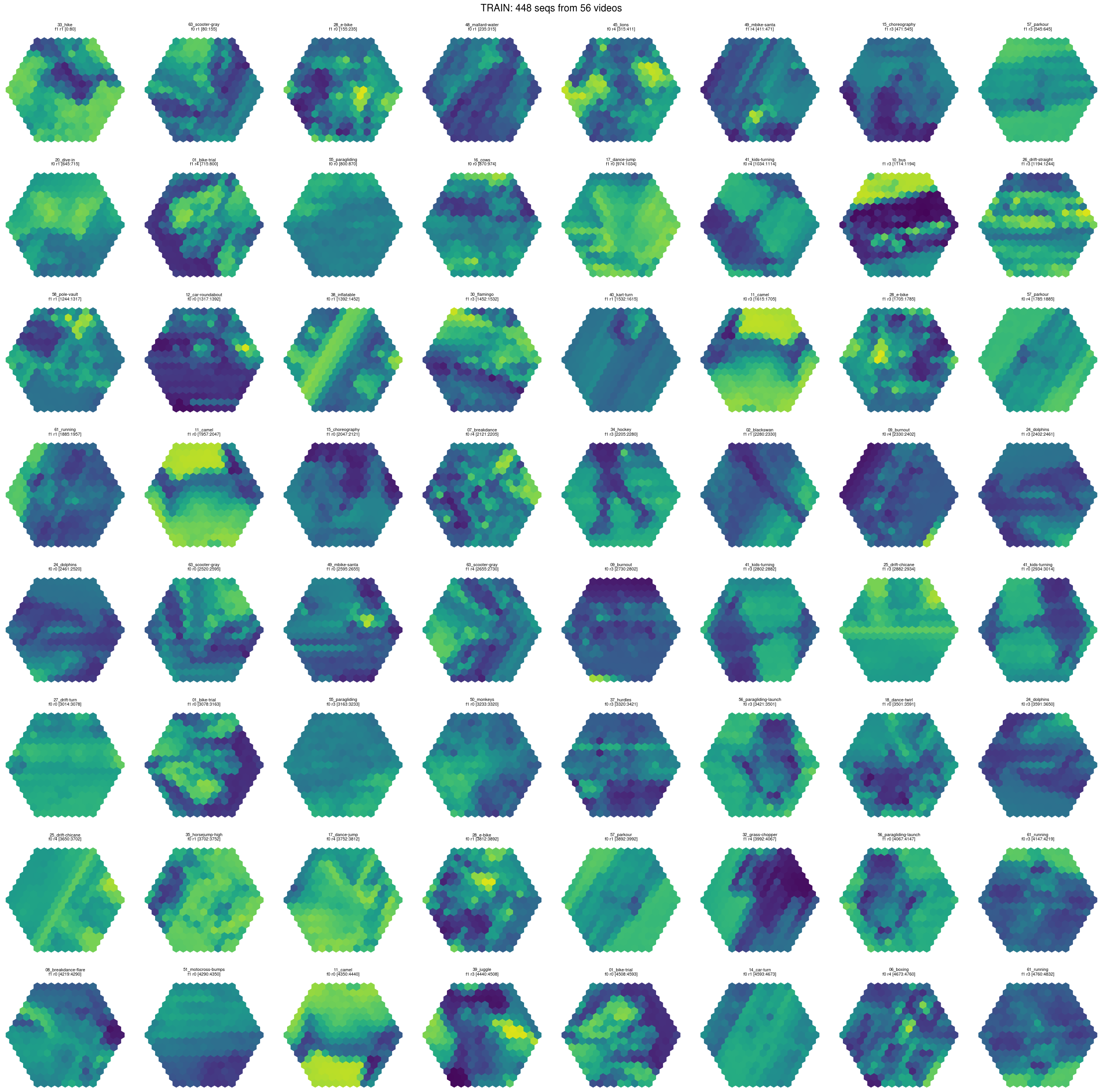
Training sequences

First frames of the shuffled DAVIS sequences assigned to training (shown for the noise-free dataset).

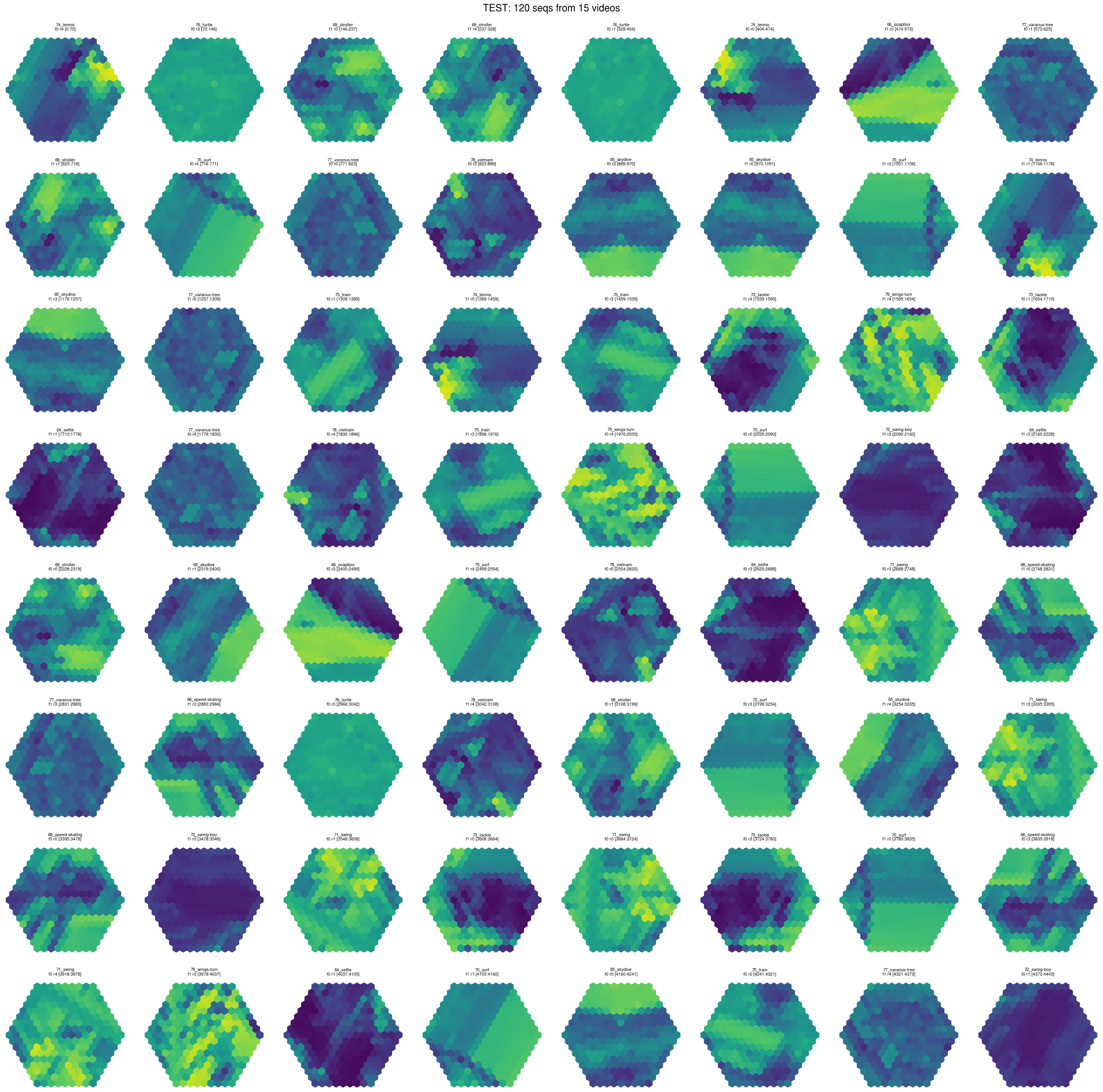
Test sequences

First frames of the shuffled DAVIS sequences assigned to testing (shown for the noise-free dataset).

Visual Stimulus Movie

The animation below shows the visual input \(I_i(t)\) as seen by the 217 hexagonal columns of the compound eye. Each hexagon represents one retinotopic column (8 photoreceptors, R1–R8, share the same input), and the color encodes the grayscale luminance at each time step. The stimulus is derived from the DAVIS natural video dataset and resampled onto the hexagonal lattice.

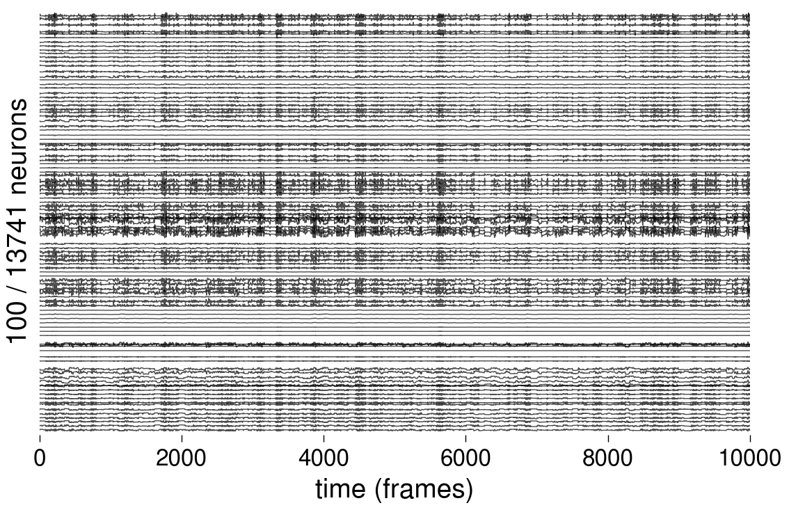
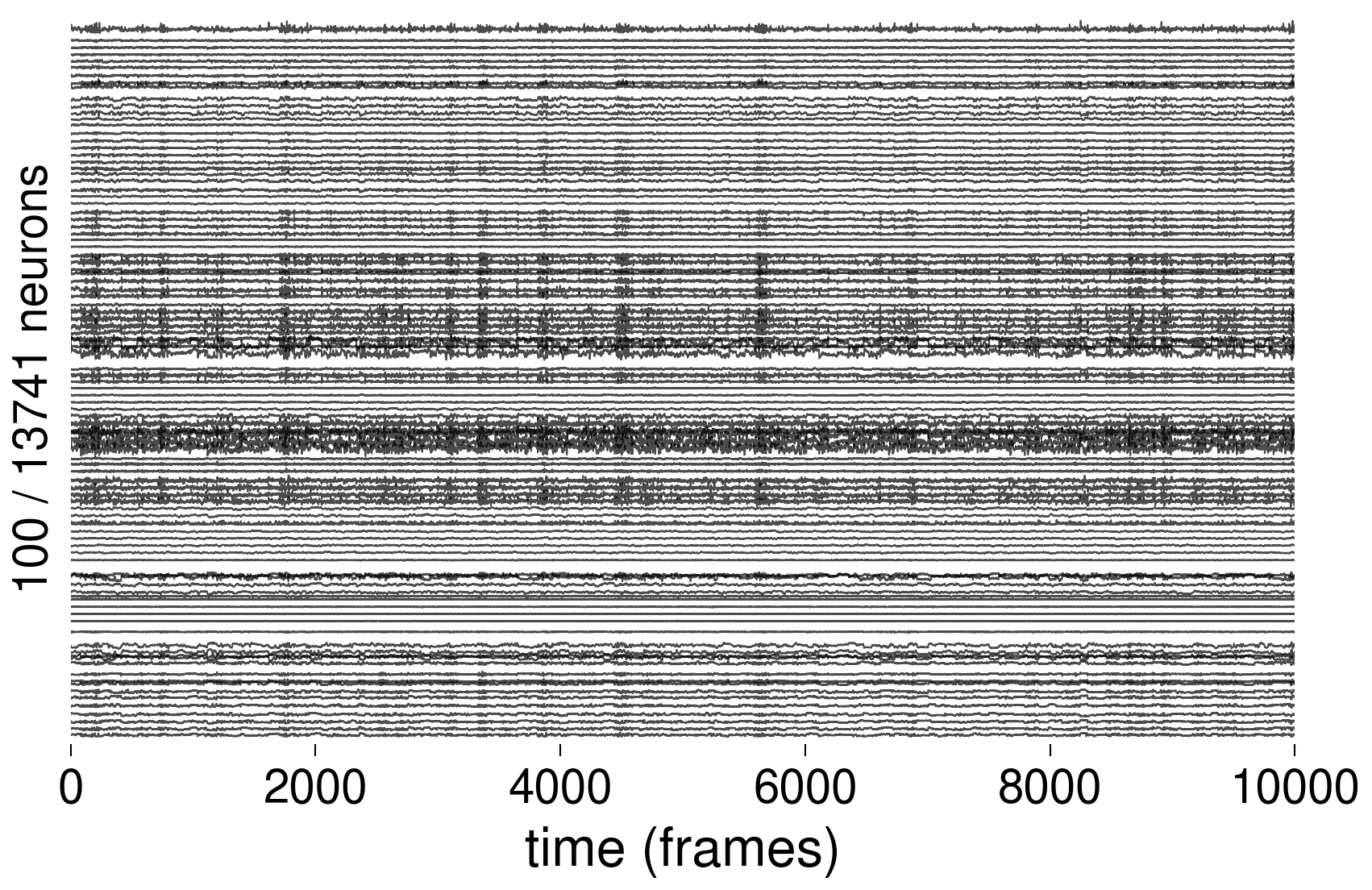
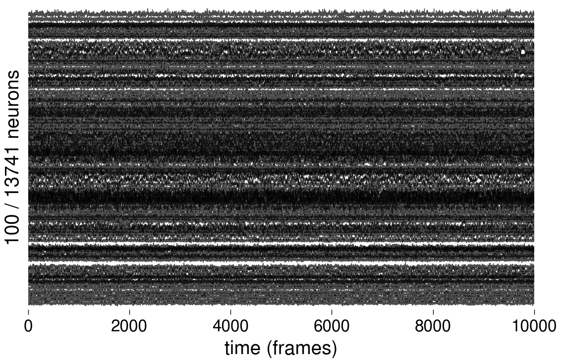
Activity Traces

Each plot below shows 100 randomly selected voltage traces \(v_i(t)\) over the first 10,000 time steps (out of 64,000 total). The three plots corresponds to the three level of intrinsinc noise used in simulations.

Noise-free (\(\sigma = 0\))

Low noise (\(\sigma = 0.05\))

High noise (\(\sigma = 0.5\))

References

[1] J. K. Lappalainen et al., “Connectome-constrained networks predict neural activity across the fly visual system,” Nature, 2024. doi:10.1038/s41586-024-07939-3

[2] D. J. Butler et al., “A Naturalistic Open Source Movie for Optical Flow Evaluation,” ECCV, 2012. doi:10.1007/978-3-642-33783-3_44

[3] F. Perazzi et al., “A Benchmark Dataset and Evaluation Methodology for Video Object Segmentation,” CVPR, 2016. doi:10.1109/CVPR.2016.85