GNN Training: Learning Circuit Dynamics

Train a message-passing GNN to approximate the circuit dynamics from voltage traces alone, learning synaptic weights, neuron embeddings, and nonlinear activation functions at each noise level.

Graph Neural Network Model

We approximated the simulated voltage dynamics by a message-passing GNN [2]:

\[\frac{\widehat{dv}_i(t)}{dt} = f_\theta\!\left(v_i(t),\,\mathbf{a}_i,\,\sum_{j\in\mathcal{N}_i} \widehat{W}_{ij}\,g_\phi\!\big(v_j(t),\,\mathbf{a}_j\big)^2,\,I_i(t)\right).\]

Nodes of the GNN correspond to neurons and edges correspond to functional synaptic connections. The GNN learned a latent embedding \(\mathbf{a}_i \in \mathbb{R}^2\) for each neuron \(i\), giving each neuron a compact latent identity to capture cell-type specific properties (like time constants and nonlinearities).

Neuron update \(f_\theta = \text{MLP}_0\) and edge message \(g_\phi = \text{MLP}_1\) are three-layer perceptrons (width 80, ReLU, linear output). \(g_\phi\) maps presynaptic inputs \(v_j\) to nonnegative messages (via squaring) depending on neural embedding \(\mathbf{a}_j\), which are weighted by \(\widehat{W}_{ij}\). \(f_\theta\) processes the postsynaptic voltage \(v_i\), aggregated input, and external input \(I_i(t)\) to predict \(\widehat{dv}_i(t)/dt\), depending on neural embedding \(\mathbf{a}_i\).

During training, inputs \(I_i(t)\), adjacency \(\mathcal{N}_i\), and activity \(v_i(t)\) are given. The MLPs, \(\widehat{W}_{ij}\), and \(\mathbf{a}_i\) are optimized by minimizing

\[\mathcal{L}_{\text{pred}} = \sum_{i,t} \|\hat{y}_i(t) - y_i(t)\|^2\]

between simulator targets \(y_i(t) = dv_i(t)/dt\) and GNN predictions \(\hat{y}_i(t) = \widehat{dv}_i(t)/dt\).

Degeneracy of the Inverse Problem

The inverse problem solved by the GNN is ill-posed: recovering five coupled components (\(\widehat{W}\), \(\tau\), \(V^{\text{rest}}\), \(f_\theta\), \(g_\phi\)) from voltage traces alone is under-determined. Many different parameter combinations can produce indistinguishable voltage predictions. This degeneracy manifests as seed dependence: slight differences in the random initialization, noise realization, or stimulus sampling can push the optimizer toward a different optimum on the degenerate solution landscape.

The regularization terms below address this degeneracy by constraining the solution space: simplicity penalties on the MLPs shrink the set of degenerate solutions, monotonicity enforces biophysical priors on \(g_\phi\), and sparsity on \(\widehat{W}\) favors connectivity patterns consistent with the true circuit. A systematic approach to quantifying and reducing degeneracy through agentic hyper-parameter optimization is presented in Notebook 09.

Regularization

We augmented the objective loss with several regularization terms:

\[\mathcal{L} = \underbrace{\lVert\widehat{\mathbf{y}}-\mathbf{y}\rVert_2}_{\text{prediction}} + \lambda_0\lVert\theta\rVert_1 + \lambda_1\lVert\phi\rVert_1 + \lambda_2\lVert\widehat{\mathbf{W}}\rVert_1 + \gamma_0\lVert\theta\rVert_2 + \gamma_1\lVert\phi\rVert_2 + \gamma_2\lVert\widehat{\mathbf{W}}\rVert_2 + \mu_0\left\lVert\mathrm{ReLU}\!\left(-\tfrac{\partial\,g_\phi}{\partial v}\right)\right\rVert_2 + \mu_1\lVert g_\phi(v_\star,\mathbf{a})-v_\star\rVert_2\]

The \(\ell_1\) and \(\ell_2\) penalties on the MLP parameters \(\theta\) and \(\phi\) act as simplicity regularizers: they bias the learned functions \(f_\theta\) and \(g_\phi\) toward simpler input–output mappings, reducing the space of degenerate solutions that fit the observed derivatives equally well. The \(\ell_1\) term (\(\lambda_2\)) additionally promotes sparsity in the connectivity matrix. The derivative term (\(\mu_0\)) enforces that the edge message \(g_\phi\) increases monotonically with voltage, and the normalization term (\(\mu_1\)) anchors \(g_\phi\) at a reference voltage \(v_\star\).

Equation term	Config key	Plot legend
\(\lambda_0\lVert\theta\rVert_1\), \(\gamma_0\lVert\theta\rVert_2\)	coeff_f_theta_weight_L1, coeff_f_theta_weight_L2	\(f_\theta\) weight regul
\(\lambda_1\lVert\phi\rVert_1\), \(\gamma_1\lVert\phi\rVert_2\)	coeff_g_phi_weight_L1, coeff_g_phi_weight_L2	\(g_\phi\) weight regul
\(\lambda_2\lVert\widehat{\mathbf{W}}\rVert_1\)	coeff_W_L1	\(\widehat{\mathbf{W}}\) \(L_1\) sparsity
\(\gamma_2\lVert\widehat{\mathbf{W}}\rVert_2\)	coeff_W_L2	\(\widehat{\mathbf{W}}\) \(L_2\) regul
\(\mu_0\) monotonicity	coeff_g_phi_diff	\(g_\phi\) monotonicity
\(\mu_1\) normalization	coeff_g_phi_norm	\(g_\phi\) norm

Annealing. The weight-based regularizers (\(L_1\)/\(L_2\) on \(\theta\), \(\phi\), and \(\widehat{\mathbf{W}}\)) are not applied at full strength from the start. Instead they follow an exponential ramp-up schedule \(c(e) = c_{\max}\,(1 - e^{-0.5\,e})\) where \(e\) is the epoch number, so the model can first learn the dynamics before regularization pressure increases. The structural penalties (\(g_\phi\) monotonicity and norm) are applied at constant strength throughout training.

MLP Architecture

Both MLPs use ReLU activations with a linear output layer. The architecture is shared across all three noise conditions except for the embedding dimension.

Component	Layers	Hidden dim	Input size	Output size	Activation
\(g_\phi\) (MLP\(_1\), edge message)	3	80	\(1 + d_\text{emb}\)	1	ReLU, squared output
\(f_\theta\) (MLP\(_0\), node update)	3	80	\(3 + d_\text{emb}\)	1	ReLU, linear output

The embedding dimension \(d_\text{emb} = 4\) for the noise-free model and \(d_\text{emb} = 2\) for both noisy conditions.

Training Parameters

We found different training hyperparameters for each of the three noise conditions. The noise-free model relied almost exclusively on the monotonicity penalty (\(\mu_0 = 1500\)) with a larger embedding dimension (\(d_\text{emb} = 4\)). At \(\sigma = 0.05\) and \(\sigma = 0.5\), \(L_1\) sparsity on the connectivity matrix and both MLPs was activated, and the \(g_\phi\) normalization term was turned on (\(\mu_1 = 0.9\)). The two noisy conditions differed mainly in that \(\sigma = 0.05\) used higher learning rates and more data augmentation (35 vs 20 loops), while \(\sigma = 0.5\) required stronger \(f_\theta\) \(L_1\) regularization (\(\lambda_0 = 0.5\) vs \(0.05\)).

Parameter	Noise-free	Noise 0.05	Noise 0.5
n_epochs	5	1	1
batch_size	2	4	2
data_augmentation_loop	20	35	20
embedding_dim	4	2	2
\(N_\text{iter}\) / epoch	128,000	112,000	128,000
\(N_\text{iter}\) total	640,000	112,000	128,000
learning_rate_W_start	6e-4	9e-4	6e-4
learning_rate_start (\(g_\phi\), \(f_\theta\))	1.8e-3	1.8e-3	1.2e-3
learning_rate_embedding_start	1.55e-3	2.3e-3	1.55e-3
coeff_g_phi_diff (\(\mu_0\))	1500	750	750
coeff_g_phi_norm (\(\mu_1\))	0	0.9	0.9
coeff_g_phi_weight_L1 (\(\lambda_1\))	0	0.28	0.28
coeff_f_theta_weight_L1 (\(\lambda_0\))	0	0.05	0.5
coeff_f_theta_weight_L2 (\(\gamma_0\))	1e-3	1e-3	1e-3
coeff_W_L1 (\(\lambda_2\))	0	1.5e-4	7.5e-5
coeff_W_L2 (\(\gamma_2\))	1.5e-6	1.5e-6	1.5e-6

GNN training

For each noise condition we trained the GNN on the full 64,000-frame dataset. At each iteration a random time frame \(k\) was sampled and the model predicted \(\widehat{dv}/dt\) from the current voltages, stimulus, and graph structure. Training proceeded for the number of iterations specified in the configuration table above.

print()
print("=" * 80)
print("TRAIN - Training GNN on fly visual system data")
print("=" * 80)

for config_name, label in datasets:
    config = configs[config_name]
    graphs_dir = graphs_dirs[config_name]
    print()
    print(f"--- {label} ---")

    model_dir = os.path.join(log_path(config.config_file), "models")
    model_exists = os.path.isdir(model_dir) and any(
        f.startswith("best_model") for f in os.listdir(model_dir)
    ) if os.path.isdir(model_dir) else False

    loss_exists = os.path.isfile(os.path.join(log_path(config.config_file), "loss_components.pt"))

    if model_exists:
        print(f"  trained model already present in {model_dir}/")
        if loss_exists:
            print("  loss_components.pt also present.")
        print("  skipping training. To retrain, delete the log folder:")
        print(f"    rm -rf {log_path(config.config_file)}")
    else:
        print(f"  training on {config.simulation.n_frames} frames")
        print(f"  {config.training.n_epochs} epochs, batch_size={config.training.batch_size}")
        print()
        data_train(config, device=device)

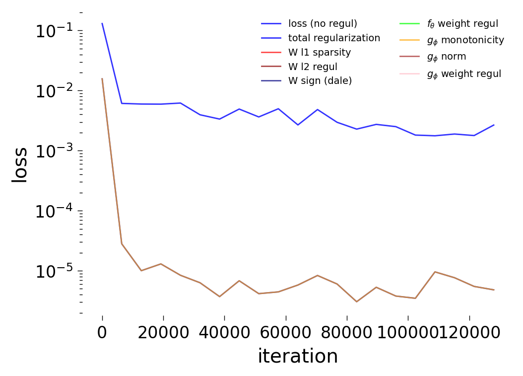
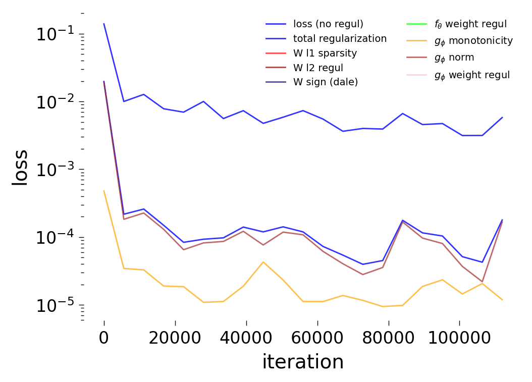
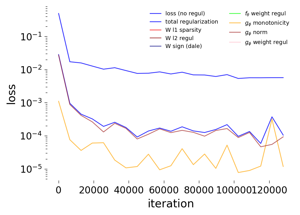
Loss Decomposition

The plots below decompose the total training loss \(\mathcal{L}\) into its constituent terms for each noise condition. Recall, the simulated dynamics include an intrinsic noise term \(\sigma\,\xi_i(t)\) where \(\xi_i(t) \sim \mathcal{N}(0,1)\) (see Notebook 00). We train the GNN at three noise levels: \(\sigma = 0\) (noise-free), \(\sigma = 0.05\) (low noise), and \(\sigma = 0.5\) (high noise).

Noise-free (\(\sigma = 0\))

Low noise (\(\sigma = 0.05\))

High noise (\(\sigma = 0.5\))

References

[1] J. K. Lappalainen et al., “Connectome-constrained networks predict neural activity across the fly visual system,” Nature, 2024. doi:10.1038/s41586-024-07939-3

[2] J. Gilmer et al., “Neural Message Passing for Quantum Chemistry,” 2017. doi:10.48550/arXiv.1704.01212