Train a SIREN implicit neural representation (INR) jointly with the GNN to recover the visual stimulus field from neural activity alone. Discuss the inherent scale/offset degeneracy and the corrected R².
Author
Allier, Lappalainen, Saalfeld
Joint Stimulus and Dynamics Recovery with GNN + INR
In the previous notebooks the visual stimulus \(I_i(t)\) was provided as a known input to the GNN. Here we ask: can the stimulus itself be recovered from neural activity alone?
We replaced the ground-truth stimulus with a learnable implicit neural representation (INR), specifically a SIREN network, that maps continuous coordinates \((t, x, y)\) to the stimulus value at each neuron position and time step. The SIREN was trained jointly with the GNN. This amounted to solving a harder inverse problem: recovering not only the circuit parameters (\(W\), \(\tau\), \(V^{\text{rest}}\), \(f_\theta\), \(g_\phi\)) but also the stimulus field from voltage data alone.
SIREN Architecture
The SIREN (Sinusoidal Representation Network) uses periodic activation functions \(\phi(x) = \sin(\omega_0 \cdot x)\) instead of ReLU, enabling it to represent fine spatial and temporal detail in the stimulus field.
The key hyperparameters explored by the agentic hyper-parameter optimization (Notebook 09) are:
\(\omega_0\) (frequency scaling): controls the spectral bandwidth of the representation. Higher \(\omega_0\) allows the network to capture faster temporal fluctuations and sharper spatial edges.
hidden_dim: network width (number of hidden units per layer).
n_layers: network depth.
learning rate: must scale inversely with \(\omega_0\) for stable training.
The input is a 3D coordinate \((t, x, y)\) normalized to the training domain, and the output is a scalar stimulus value for each neuron at each time step.
Scale/Offset Degeneracy and Corrected \(R^2\)
The SIREN output enters the GNN through \(f_\theta\), which receives the concatenated input \([v_i,\, \mathbf{a}_i,\, \text{msg}_i,\, I_i(t)]\). This creates an inherent scale/offset degeneracy: \(f_\theta\)’s biases absorb any constant offset, and its weights on the excitation dimension compensate any scale factor (including sign inversion). The SIREN and \(f_\theta\) jointly optimize along a degenerate manifold where the stimulus pattern is learned correctly but the linear mapping between SIREN output and true stimulus is unidentifiable. We therefore apply a global linear fit\(I^{\text{true}} = a \cdot I^{\text{pred}} + b\) and report the corrected \(R^2\).
Noise Level
Recall that the simulated dynamics include an intrinsic noise term \(\sigma\,\xi_i(t)\) where \(\xi_i(t) \sim \mathcal{N}(0,1)\) (Notebook 00). The joint GNN+INR experiment presented here uses \(\sigma = 0.05\) (low noise). To change the noise level, edit the noise_model_level field in the config file config/fly/flyvis_noise_005_INR.yaml.
Results
The joint GNN+SIREN model uses the flyvis_noise_005_INR config, which extends the noise 0.05 setup with SIREN parameters (hidden_dim=2048, 4 layers, \(\omega_0\)=4096). Training alternates between full GNN learning rates in epoch 0 and reduced rates (x0.05) in subsequent epochs, while the SIREN learning rate remains constant.
Despite the added complexity of jointly learning the stimulus field, the GNN still recovers synaptic weights, time constants, resting potentials, and neuron-type embeddings with quality comparable to the known-stimulus baseline.
Data Generation
The INR config uses the same flyvis_noise_005 simulation data. If it has not been generated yet (via Notebook 00), we generate it here.
Code
data_exists = os.path.isdir(os.path.join(graphs_dir, 'x_list_train')) or\ os.path.isdir(os.path.join(graphs_dir, 'x_list_0'))if data_exists:print(f"Data already exists at {graphs_dir}/")print("Skipping simulation.")else:print(f"Generating simulation data for {config_name}...") data_generate( config, device=device, visualize=False, run_vizualized=0, style="color", alpha=1, erase=True, save=True, step=100, )
Training
The joint GNN+SIREN model is trained end-to-end. The GNN learns synaptic weights, embeddings, and MLPs while the SIREN learns to reconstruct the stimulus field from \((t,x,y)\) coordinates. Training uses 3 epochs with alternate training: full GNN learning rates in epoch 0, then 0.05x in epochs 1+.
Code
model_dir = os.path.join(gnn_log_dir, "models")model_exists = os.path.isdir(model_dir) andany( f.startswith("best_model") for f in os.listdir(model_dir)) if os.path.isdir(model_dir) elseFalseif model_exists:print(f"Trained model already present in {model_dir}/")print("Skipping training. To retrain, delete the log folder:")print(f" rm -rf {gnn_log_dir}")else:print(f"Training joint GNN+SIREN model ({config_name})...") data_train(config=config, erase=True, device=device)
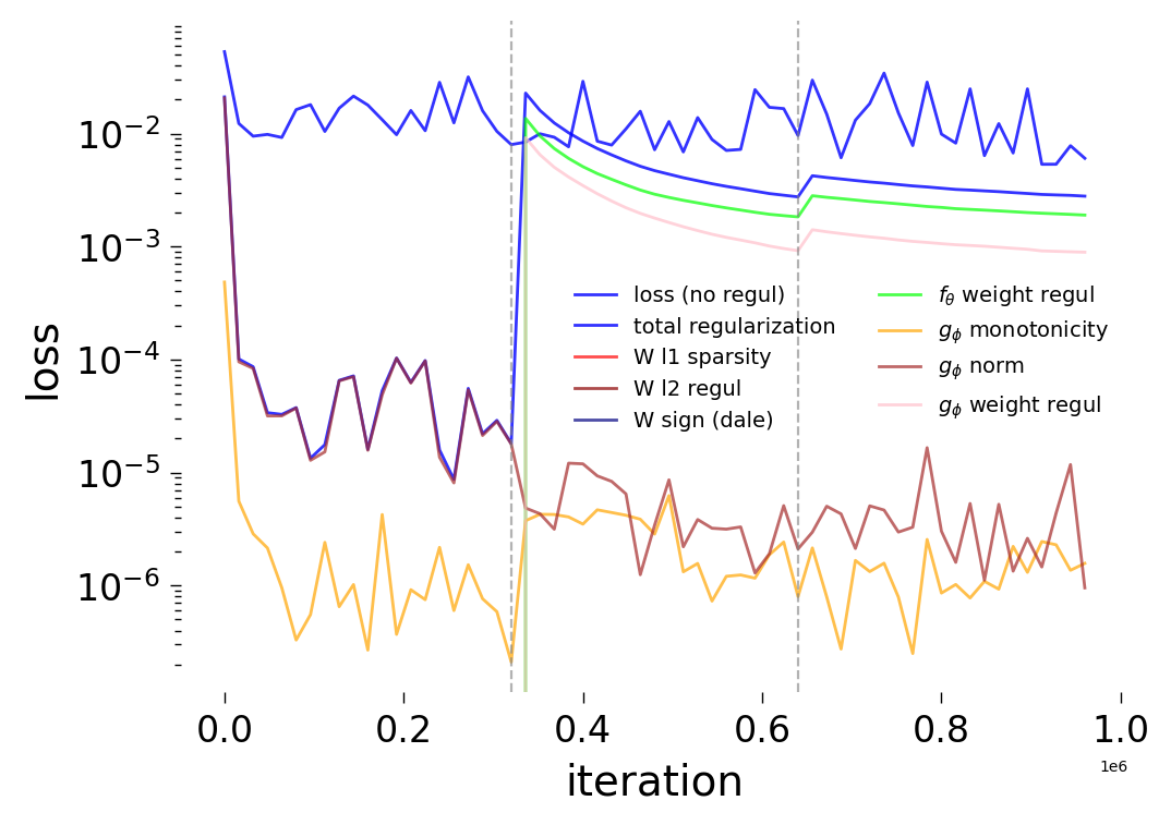
Loss Decomposition
Testing: Rollout and Stimulus Recovery
We run data_test on the joint model. For INR models, the rollout uses training data (since the SIREN was fit to it) and additionally computes the corrected stimulus \(R^2\) and generates a GT vs Pred video showing the recovered stimulus on the hexagonal photoreceptor array.
Code
print("\n--- Testing joint GNN+SIREN model ---")data_test( config=config, visualize=True, style="color name continuous_slice", verbose=False, best_model='best', run=0, step=10, n_rollout_frames=250, device=device,)
Stimulus Recovery Video
The video below shows the SIREN result with three panels:
Left: ground-truth stimulus on the hexagonal photoreceptor array.
Center: SIREN prediction after global linear correction (\(I^{\text{true}} = a \cdot I^{\text{pred}} + b\)).
Right: rolling voltage traces for selected neurons (ground truth in green, prediction in black).