GNN Testing: Robustness to Edge Removal

Test whether the GNN has learned the circuit’s computational rules by randomly ablating 50% of synaptic connections and comparing the model’s predictions to the simulator under the same reduced connectivity.

Ablation

A well-trained dynamical model should capture the circuit’s computational rules, not merely memorize its specific activities.
To test this, we randomly ablated 50% of the synaptic connections and regenerated the ground truth under the ablated connectivity. The same edge mask is then applied to the GNN’s learned weights \(\widehat{W}_{ij}\), so both the simulator and the model operate on identical reduced circuits. If the GNN has learned the correct message-passing functions \(f_\theta\) and \(g_\phi\), it should generalize to the reduced connectivity without retraining. We tested robustness at three noise levels: \(\sigma = 0\) (noise-free), \(\sigma = 0.05\) (low noise), and \(\sigma = 0.5\) (high noise). The test is performed using the best models in (Notebook 01).

Generate Ablated Data

For each noise condition, the simulator regenerates voltage traces with 50% of edges randomly zeroed. he resulting ablation mask (a boolean tensor indicating which edges survive) is saved alongside the data so that the exact same mask can be applied to the GNN’s learned weights at test time. This ensures a fair comparison: both the ground-truth simulator and the learned model operate on precisely the same reduced circuit.

print()
print("=" * 80)
print("GENERATE - data with 50% edge ablation")
print("=" * 80)

for config_name, label in mask_datasets:
    config = mask_configs[config_name]
    graphs_dir = graphs_data_path(config.dataset)
    mask_path = os.path.join(graphs_dir, "ablation_mask.pt")
    has_test_data = (os.path.isfile(os.path.join(graphs_dir, "x_list_test.pt"))
                     or os.path.isfile(os.path.join(graphs_dir, "x_list_test.npy"))
                     or os.path.isdir(os.path.join(graphs_dir, "x_list_test")))

    if os.path.exists(mask_path) and has_test_data:
        print(f"\n--- {label} ---")
        print(f"  ablated data already exists at {graphs_dir}/")
        print("  skipping generation...")
    else:
        print(f"\n--- {label} ---")
        print(f"  generating with ablation_ratio={config.simulation.ablation_ratio}")
        data_generate(config, device=device, visualize=False, style='color')

Test: GNN on Ablated Data

Each model, trained on the full non-ablated connectivity, is now evaluated on the ablated test data. Before evaluation, the saved ablation mask is loaded and applied to the model’s learned weight vector \(\widehat{\mathbf{W}}\), zeroing out the same edges that were removed in the simulator. No retraining or fine-tuning is performed; the model must rely on the message-passing functions it learned from the original circuit.

print()
print("=" * 80)
print("TEST - GNN models on ablated data")
print("=" * 80)

# Check that trained models exist for all base configs
pairs = list(zip(base_datasets, mask_datasets))
missing_models = []
for base_name, base_label in base_datasets:
    log_dir = log_path(base_configs[base_name].config_file)
    model_files = glob.glob(f"{log_dir}/models/best_model_with_*.pt")
    if not model_files:
        missing_models.append(base_label)

if missing_models:
    msg = ", ".join(missing_models)
    raise RuntimeError(
        f"No trained models found for: {msg}. "
        f"Please run Notebook_01 first to train the GNN models."
    )

for (base_name, base_label), (mask_name, mask_label) in pairs:
    print(f"\n--- {base_label} model on ablated data ---")
    data_test(
        base_configs[base_name],
        best_model='best',
        device=device,
        test_config=mask_configs[mask_name],
    )

Ablation Rollout Traces

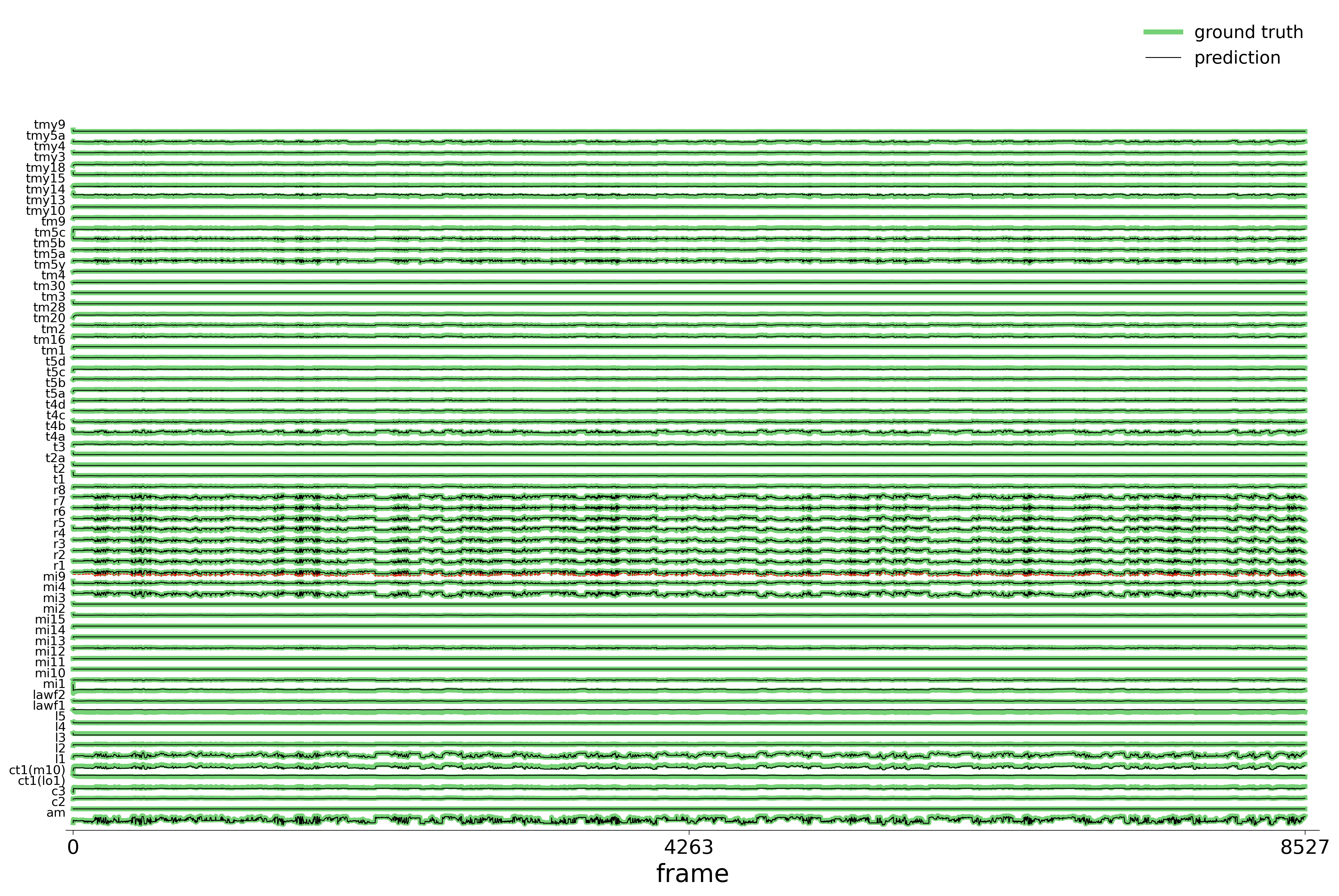
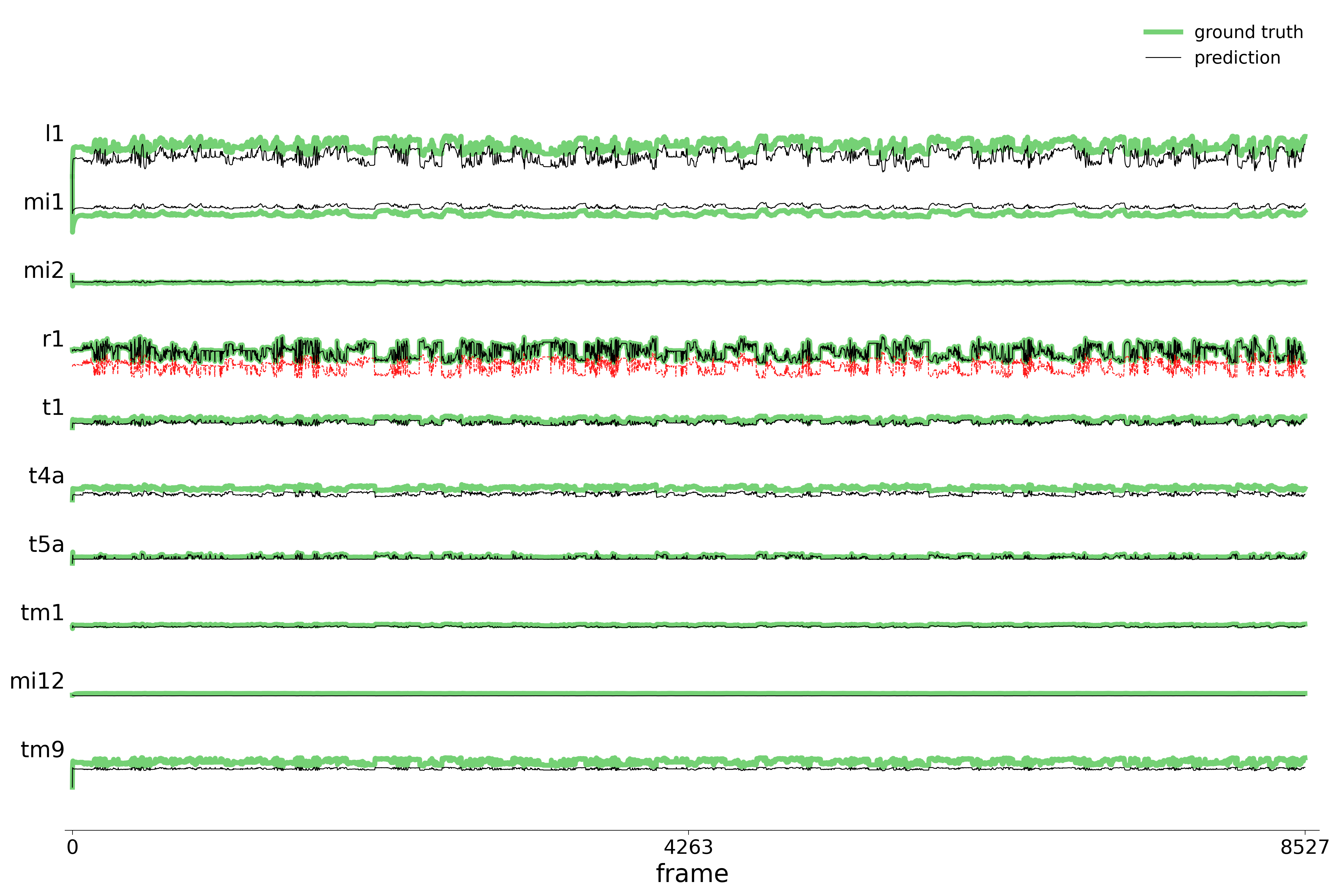
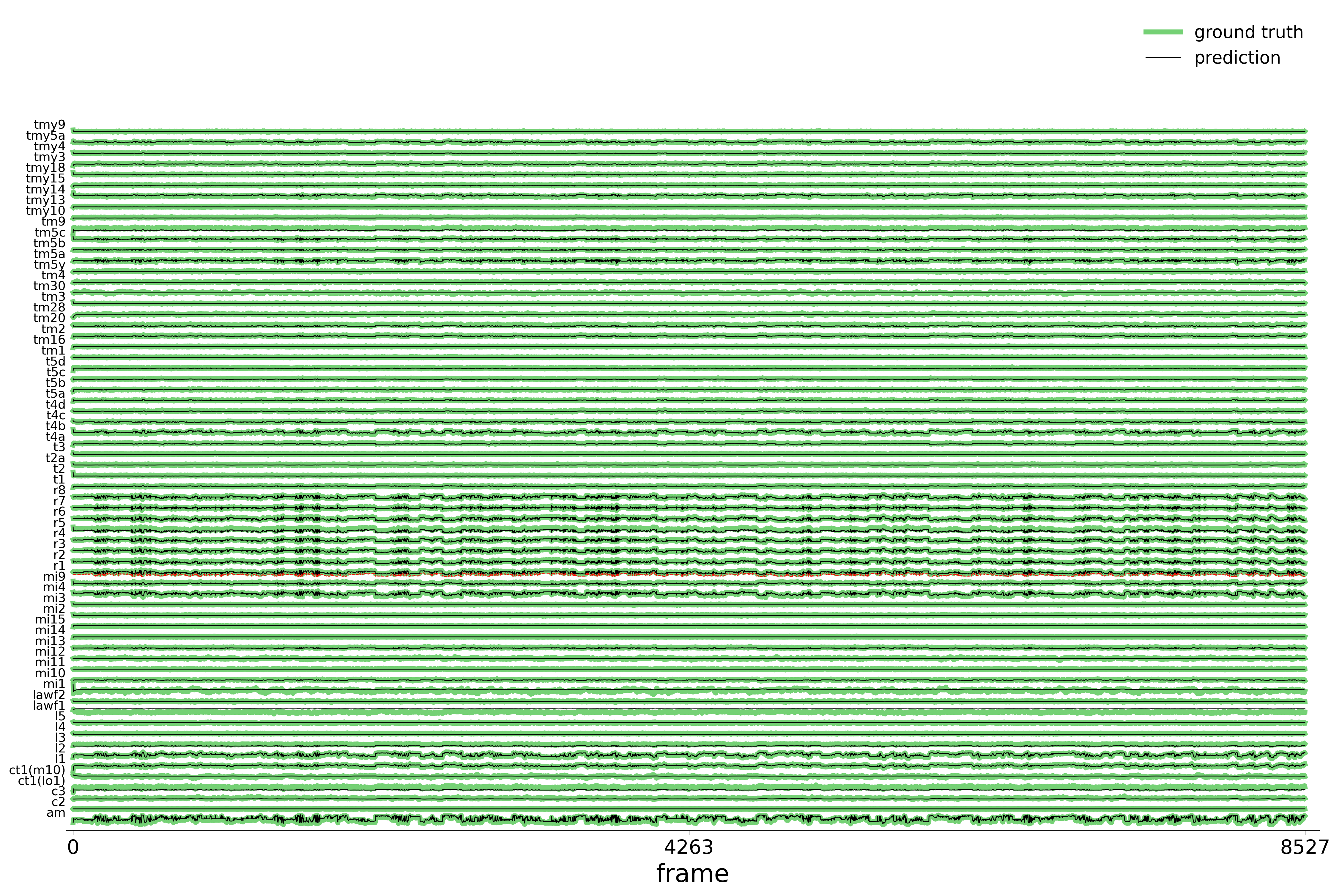
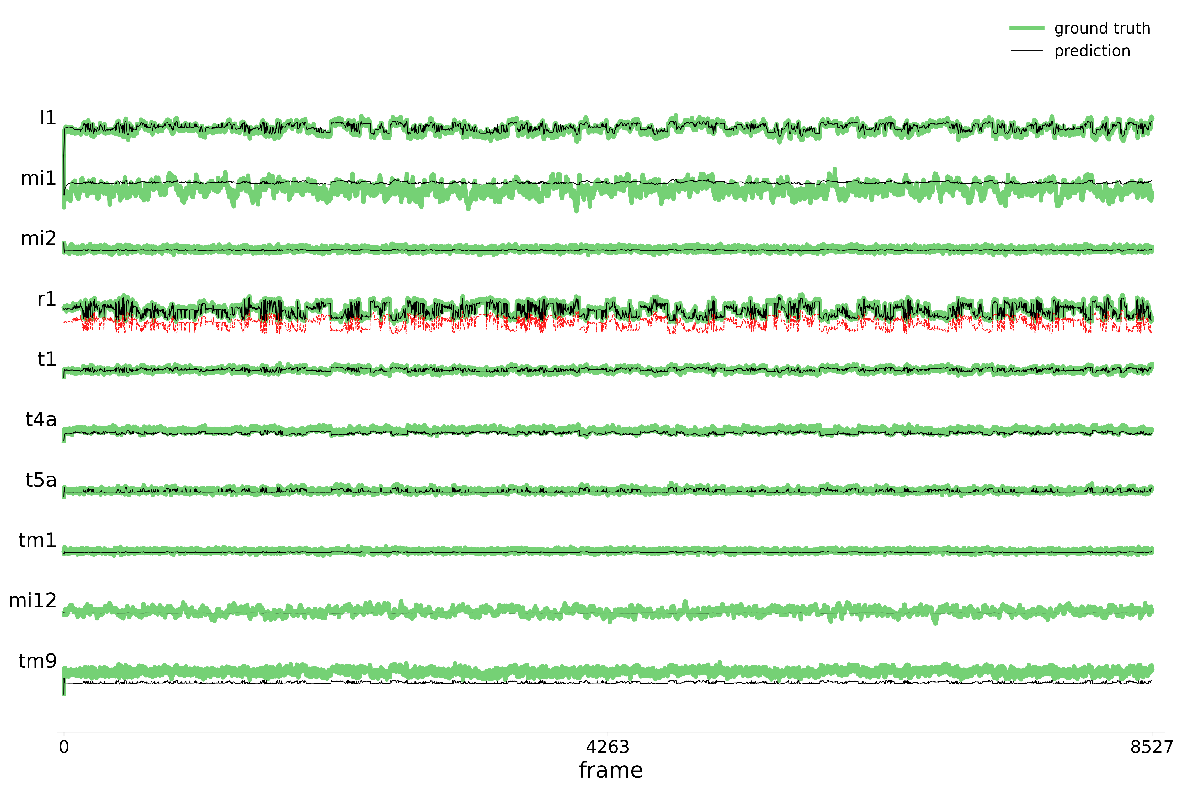
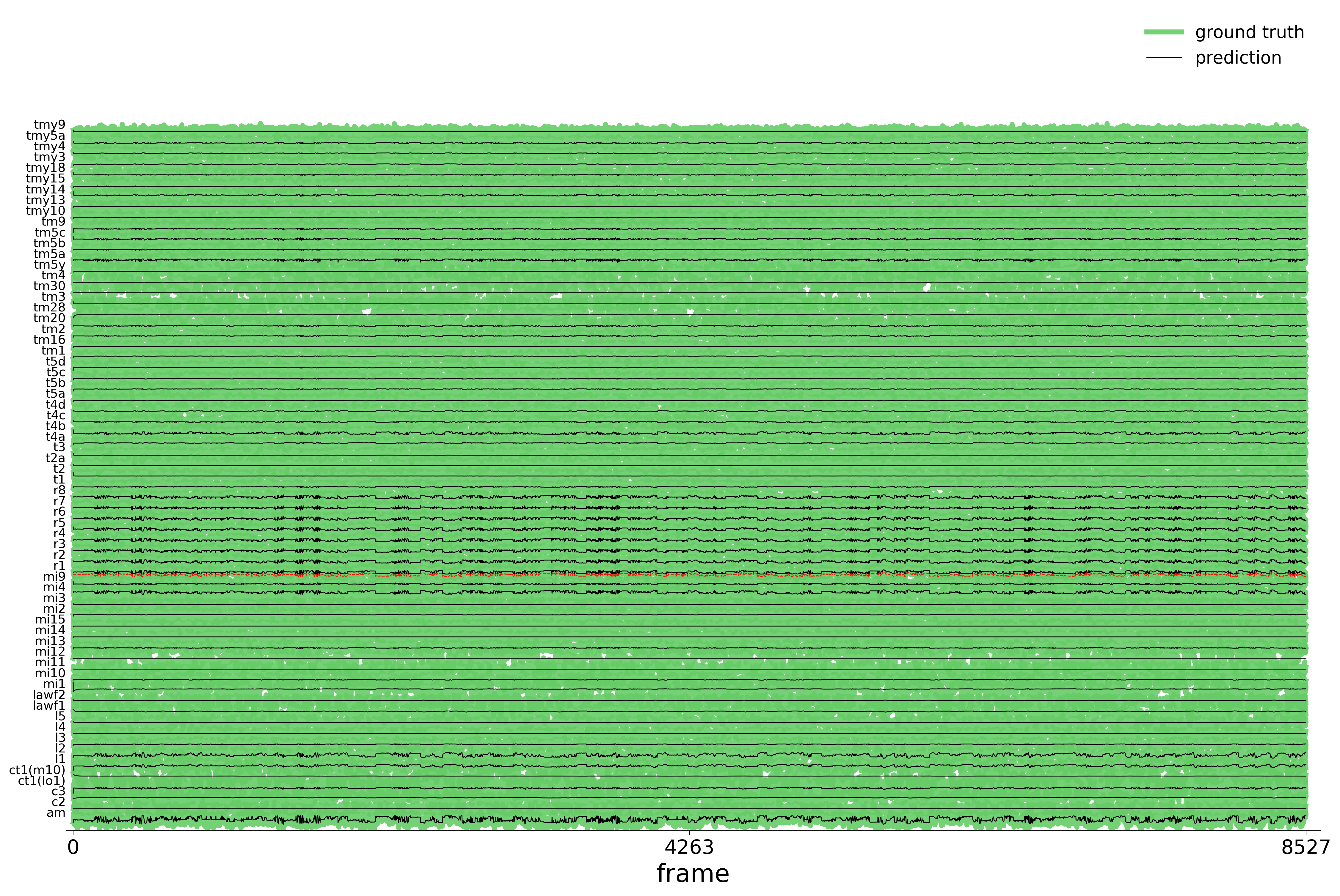
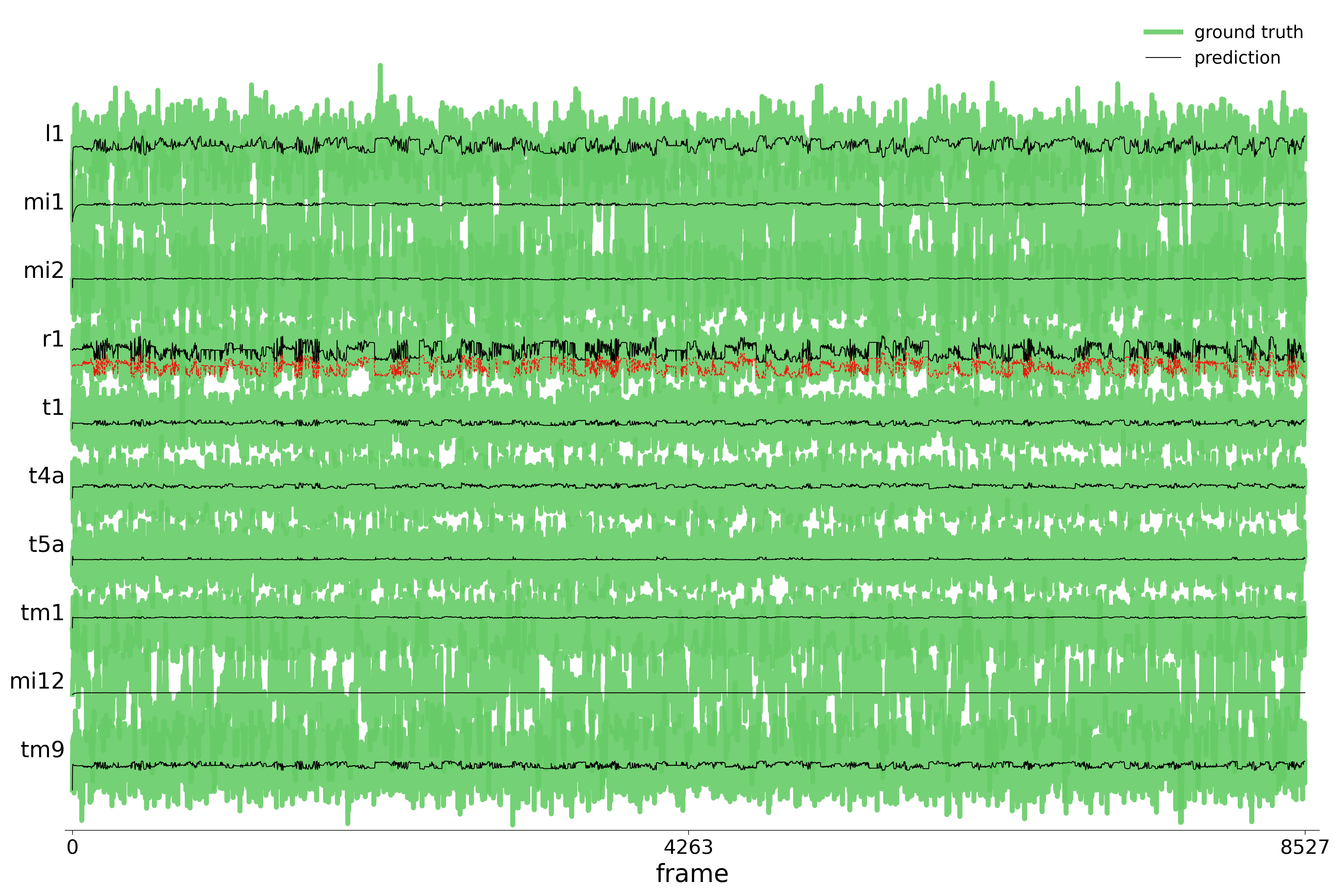
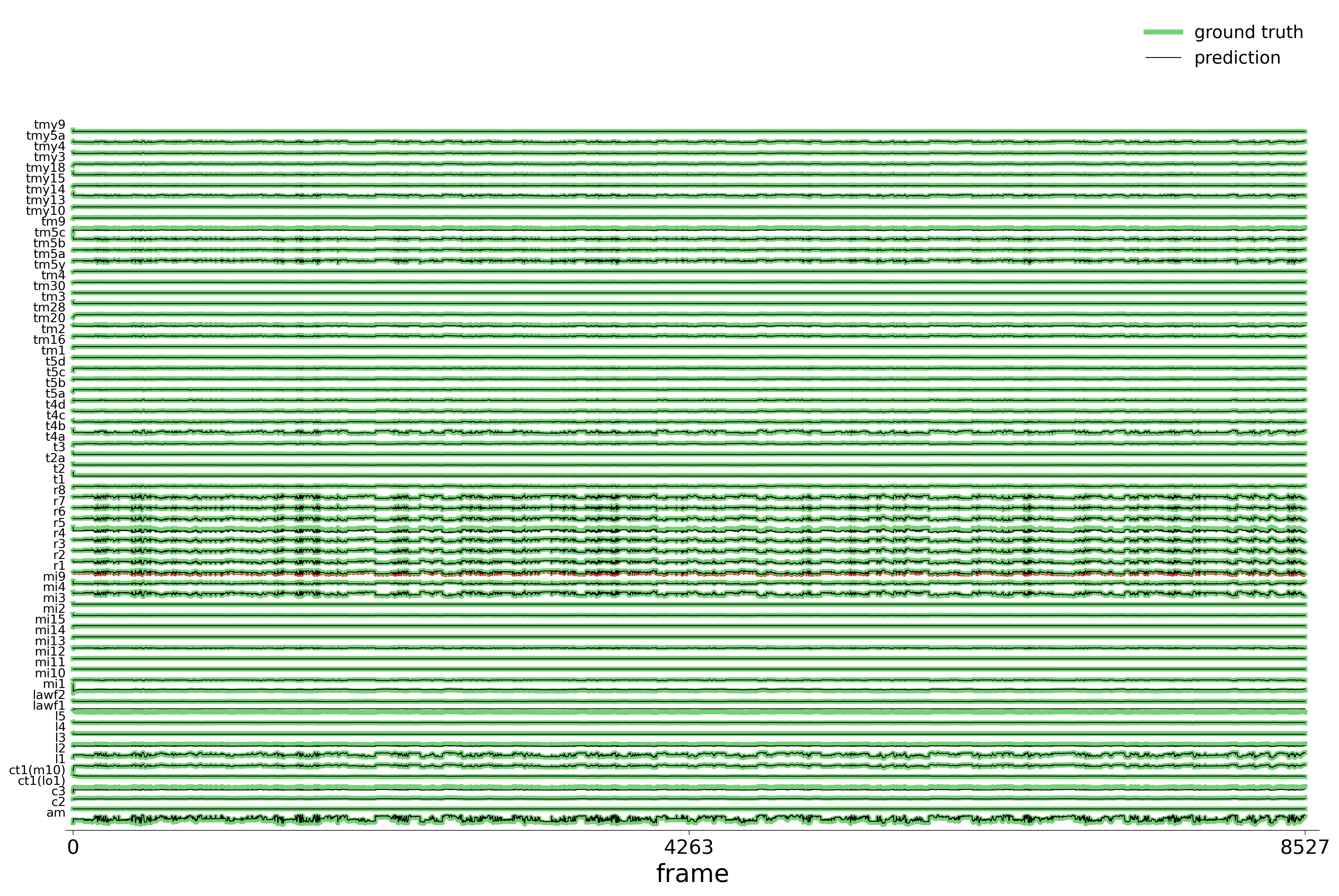
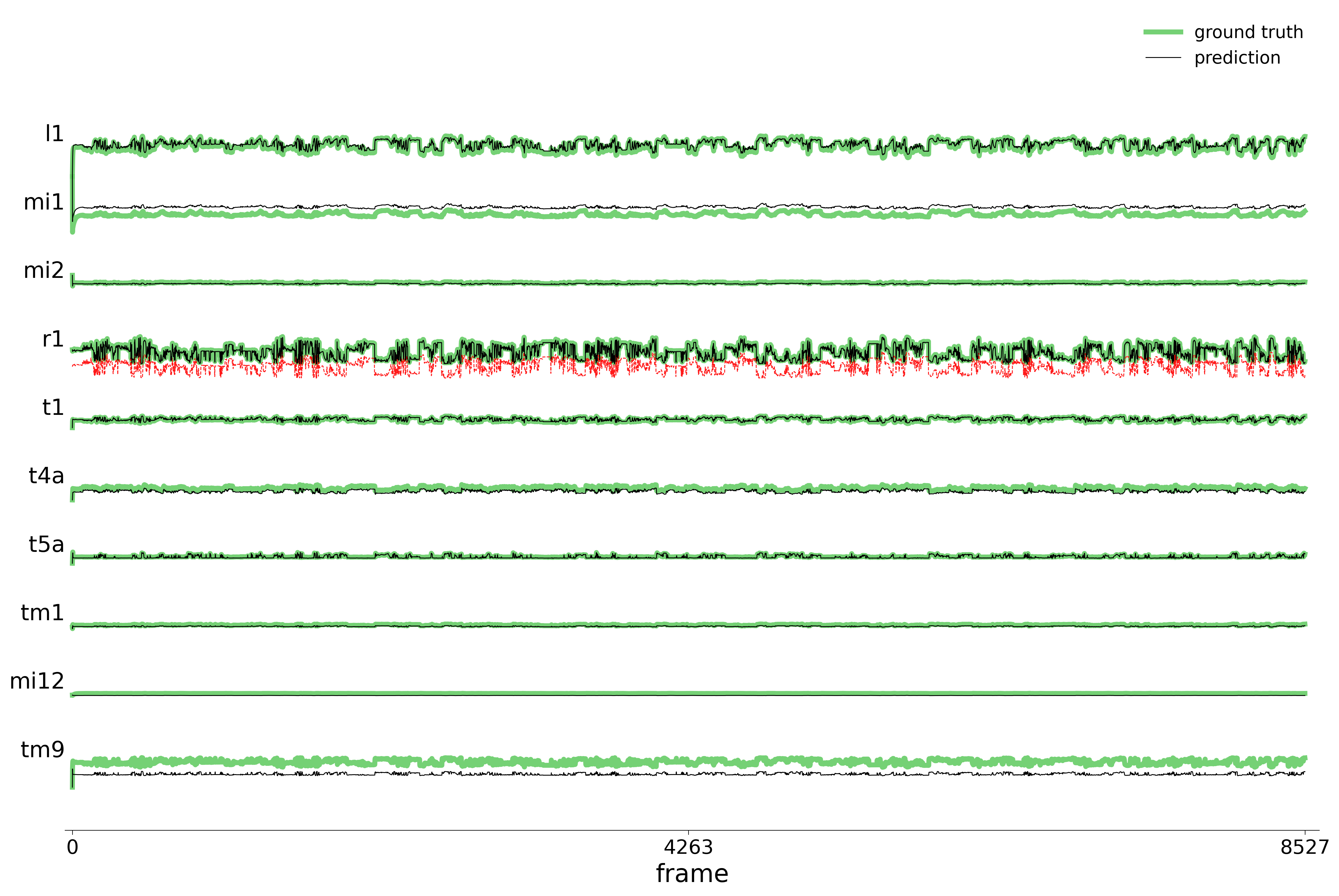
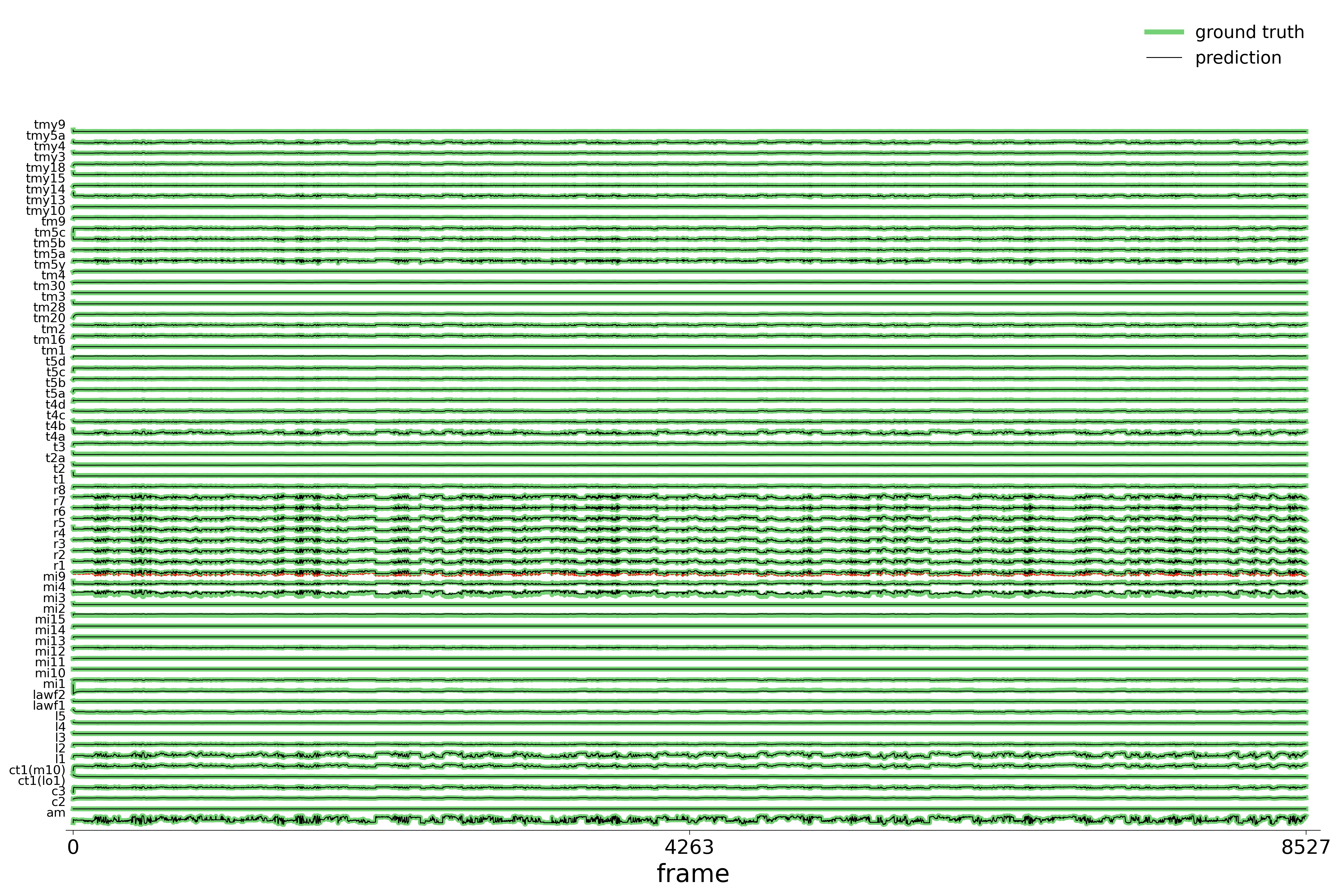
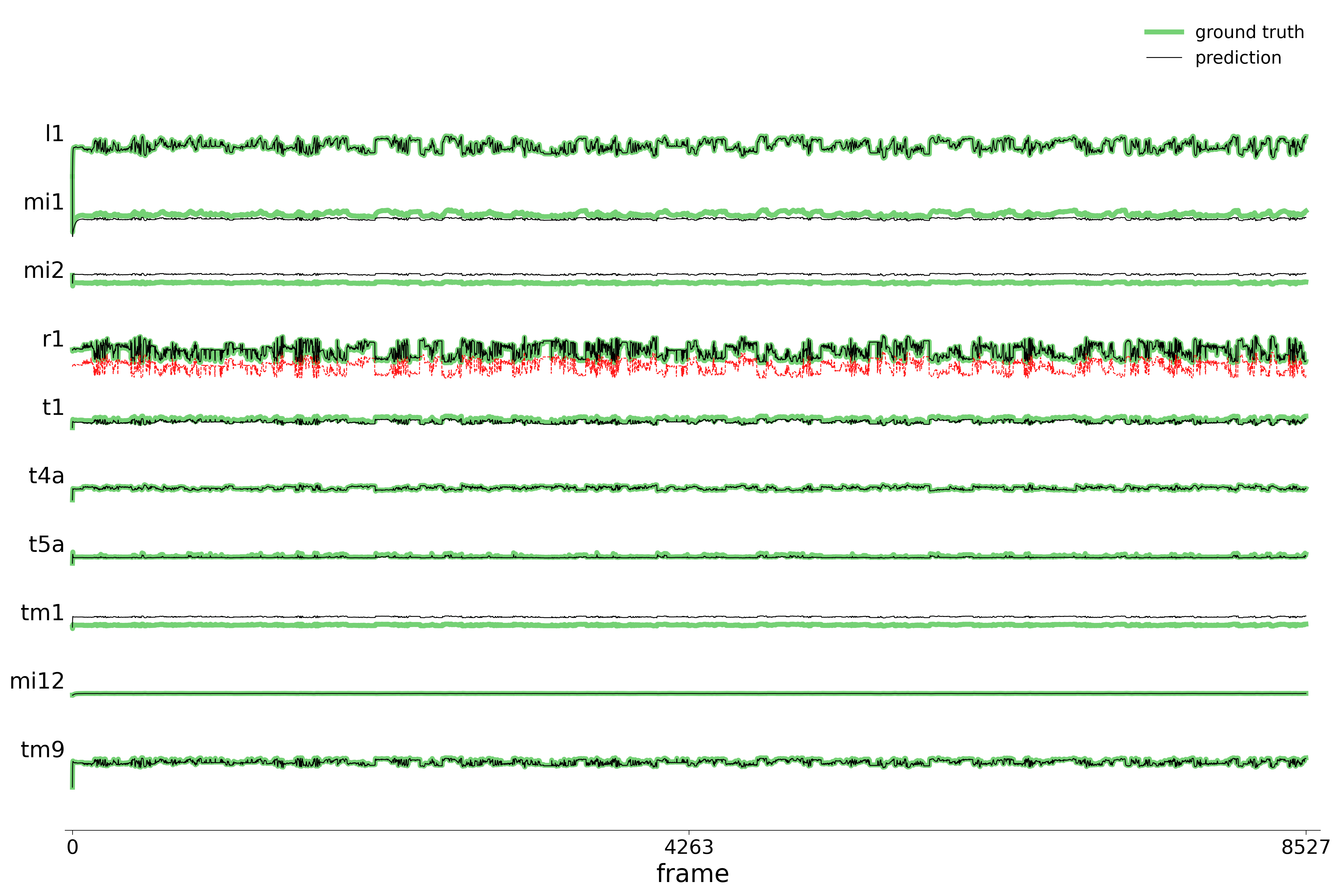
The rollout plots below compare ground-truth voltages (green) and GNN predictions (black) under 50% edge ablation. The red trace corresponds to one of the R1–R6 outer photoreceptors, which receive the visual stimulus directly from the compound eye and also integrate excitatory feedback from lamina interneurons (L2, L4, and amacrine cells). The all-types plot shows one representative neuron per cell type (65 traces), providing a global view of how the ablated GNN captures the circuit dynamics. The selected plot zooms into a subset for more detailed inspection.

Noise-free (\(\sigma = 0\))

Low noise (\(\sigma = 0.05\))

High noise (\(\sigma = 0.5\))

Ablation Metrics

The tables below report RMSE and Pearson \(r\) (mean \(\pm\) std over neurons) for the ablated evaluation, for both one-step prediction and autoregressive rollout.

One-Step Prediction (ablated data)

Metric	Noise-free	Noise 0.05	Noise 0.5
RMSE	4.6545 +/- 6.3482	2.5264 +/- 4.5307	0.9656 +/- 2.1513
Pearson r	0.944 +/- 0.125	0.989 +/- 0.042	1.000 +/- 0.002

Autoregressive Rollout (ablated data)

Metric	Noise-free	Noise 0.05	Noise 0.5
RMSE	0.1923 +/- 0.2242	0.1511 +/- 0.1582	0.7047 +/- 0.2768
Pearson r	0.932 +/- 0.180	0.559 +/- 0.338	0.129 +/- 0.142

Noise-Free Ablation Evaluation

As in the non-ablated case (Notebook 02), we cross-test the noisy models on clean data to verify that the denoising property is preserved under ablation. The models trained on noisy data (\(\sigma{=}0.05\) and \(\sigma{=}0.5\)) are evaluated on the noise-free ablated test data. If the GNN has learned the deterministic dynamics, it should still track the clean ground truth even after losing half its synaptic connections.

noise_free_mask_config = mask_configs['flyvis_noise_free_mask_50']
noisy_base = [ds for ds in base_datasets if ds[0] != 'flyvis_noise_free']

for base_name, base_label in noisy_base:
    print()
    print(f"--- {base_label} model on noise-free ablated data ---")
    data_test(
        base_configs[base_name],
        best_model='best',
        device=device,
        test_config=noise_free_mask_config,
    )

Rollout: Noisy Models on Noise-Free Ablated Data

Low noise (\(\sigma = 0.05\)) on noise-free ablated data

High noise (\(\sigma = 0.5\)) on noise-free ablated data

Noise-Free Ablation Metrics

Metric	Noise 0.05	Noise 0.5
RMSE	0.1171 +/- 0.1660	0.0516 +/- 0.0653
Pearson r	0.945 +/- 0.169	0.971 +/- 0.175

Denoising Under Ablation

The results confirm that the implicit denoising property observed in Notebook 02 is preserved under ablation. Models trained on noisy data still recover the deterministic dynamics when evaluated on noise-free ablated data, tracking the clean ground truth closely. This is a strong indication that the GNN has learned the true message-passing computation. The functions \(f_\theta\) and \(g_\phi\) generalize across both noise conditions and connectivity perturbations, rather than being overfitted to the specific training dataset.

References

[1] J. K. Lappalainen et al., “Connectome-constrained networks predict neural activity across the fly visual system,” Nature, 2024. doi:10.1038/s41586-024-07939-3

[2] J. Gilmer et al., “Neural Message Passing for Quantum Chemistry,” 2017. doi:10.48550/arXiv.1704.01212