Evaluate the trained GNN on held-out test stimuli never seen during training, comparing one-step predictions and multi-step rollouts against the ground-truth simulator trajectories.
Author
Allier, Lappalainen, Saalfeld
Test
Test Data Generation
The test set is generated from a separate pool of DAVIS video stimuli. During data generation (Notebook 00), the 71 DAVIS video subdirectories are split 80/20: 56 videos are used for training and 15 for testing. All augmentations (flips, rotations) of a given video stay in the same split, so the test visual stimuli are entirely unseen during training. The simulator then generates new voltage traces from these test stimuli using the same connectivity and dynamics parameters (see the train/test first-frame previews in Notebook 00). Recall that the simulated dynamics include an intrinsic noise term \(\sigma\,\xi_i(t)\) where \(\xi_i(t) \sim \mathcal{N}(0,1)\).
We evaluated the GNN at three noise levels: \(\sigma = 0\) (noise-free), \(\sigma = 0.05\) (low noise), and \(\sigma = 0.5\) (high noise).
Configuration
Code
print()print("="*80)print("TEST - Evaluating on new test data (unseen stimuli)")print("="*80)for config_name, label in datasets: config = configs[config_name]print()print(f"--- {label} ---") data_test(config, best_model='best', device=device)
Rollout Results
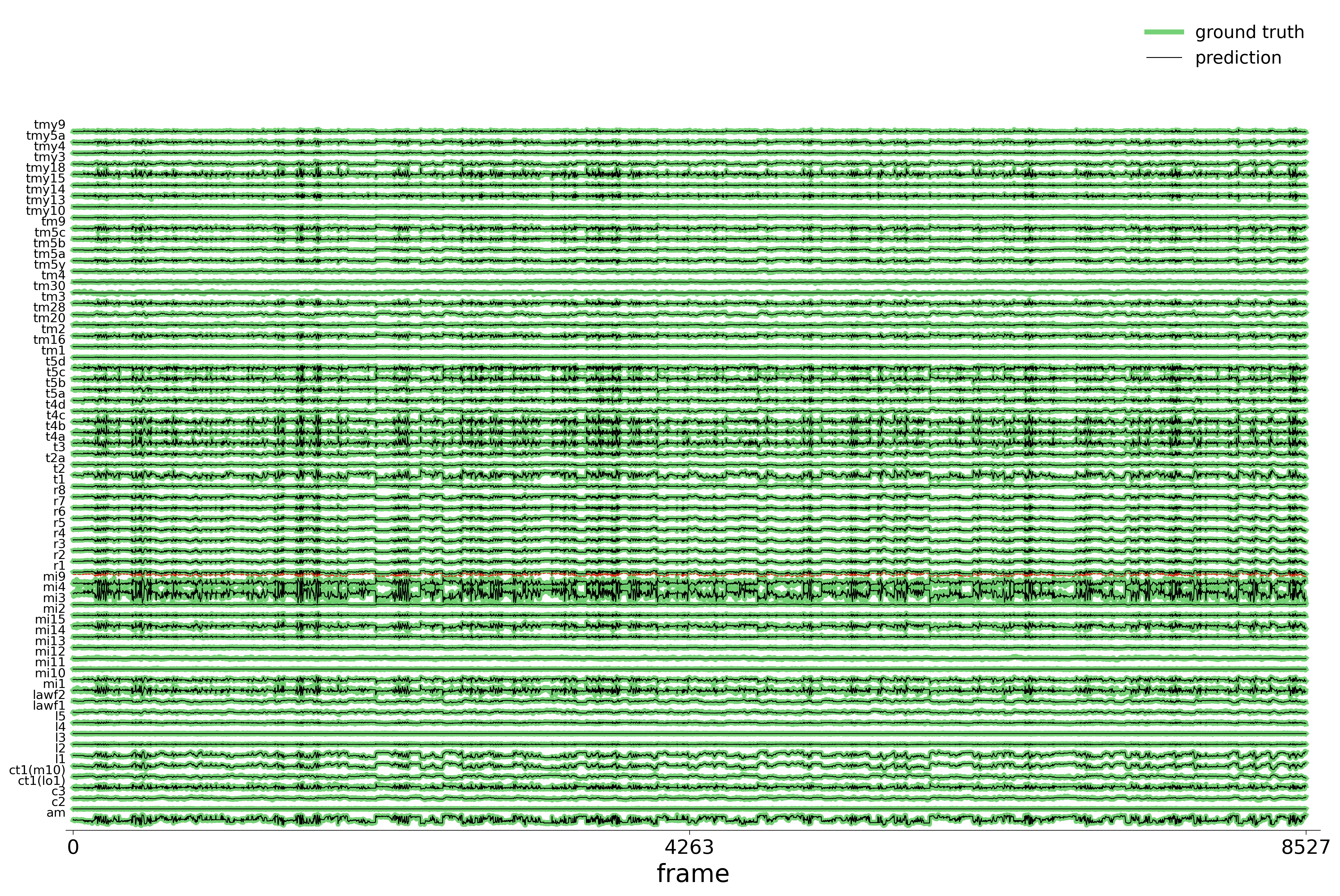
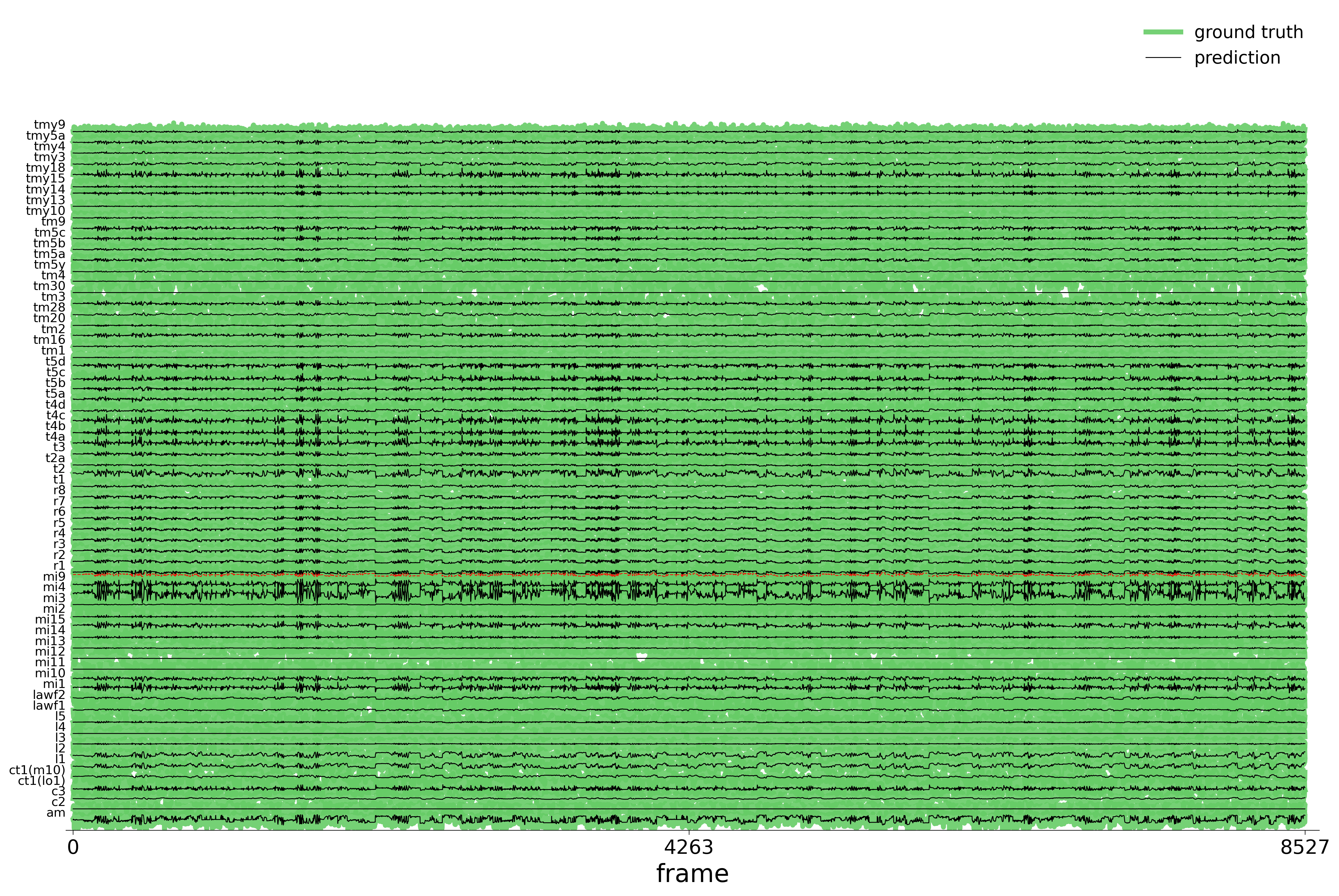
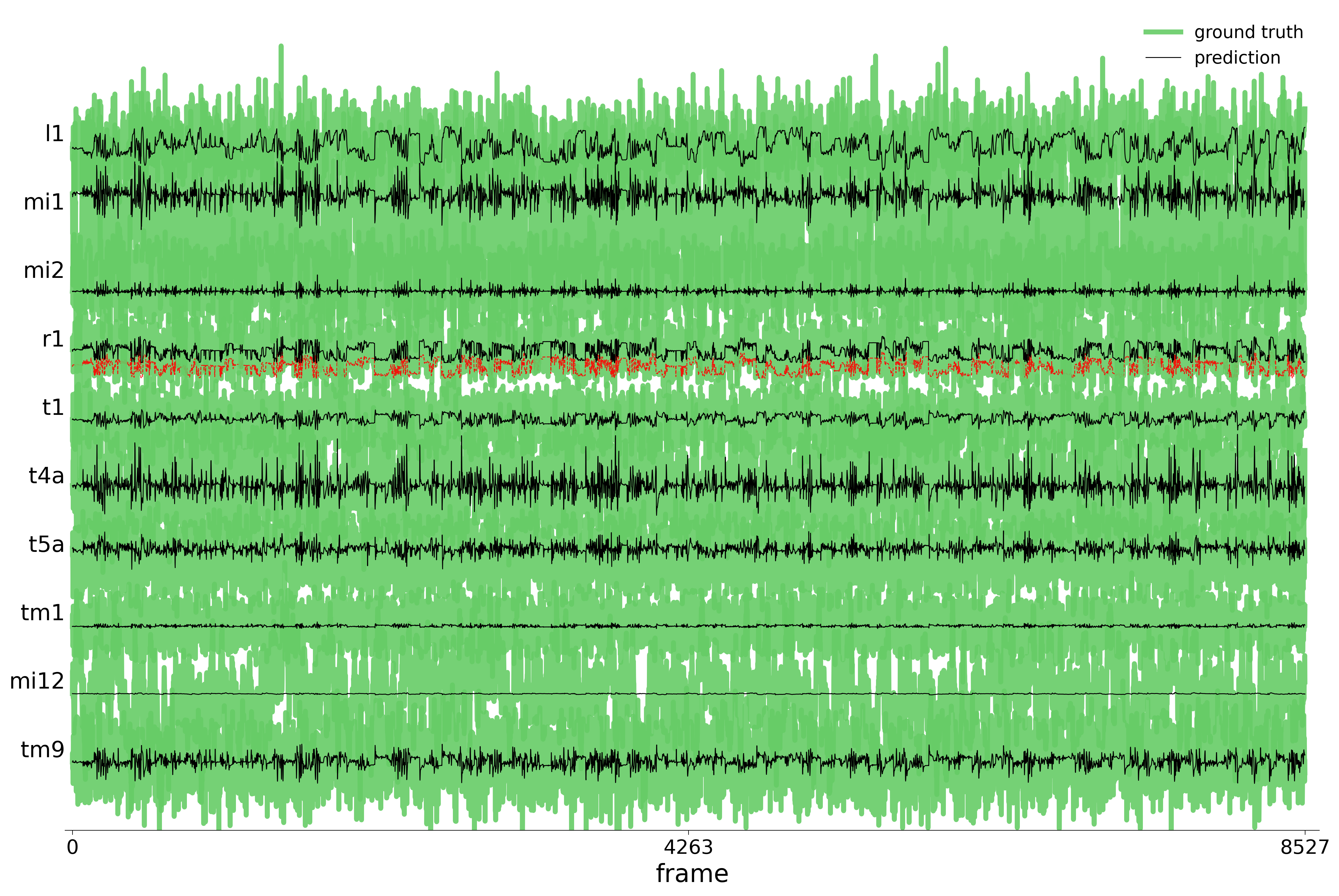
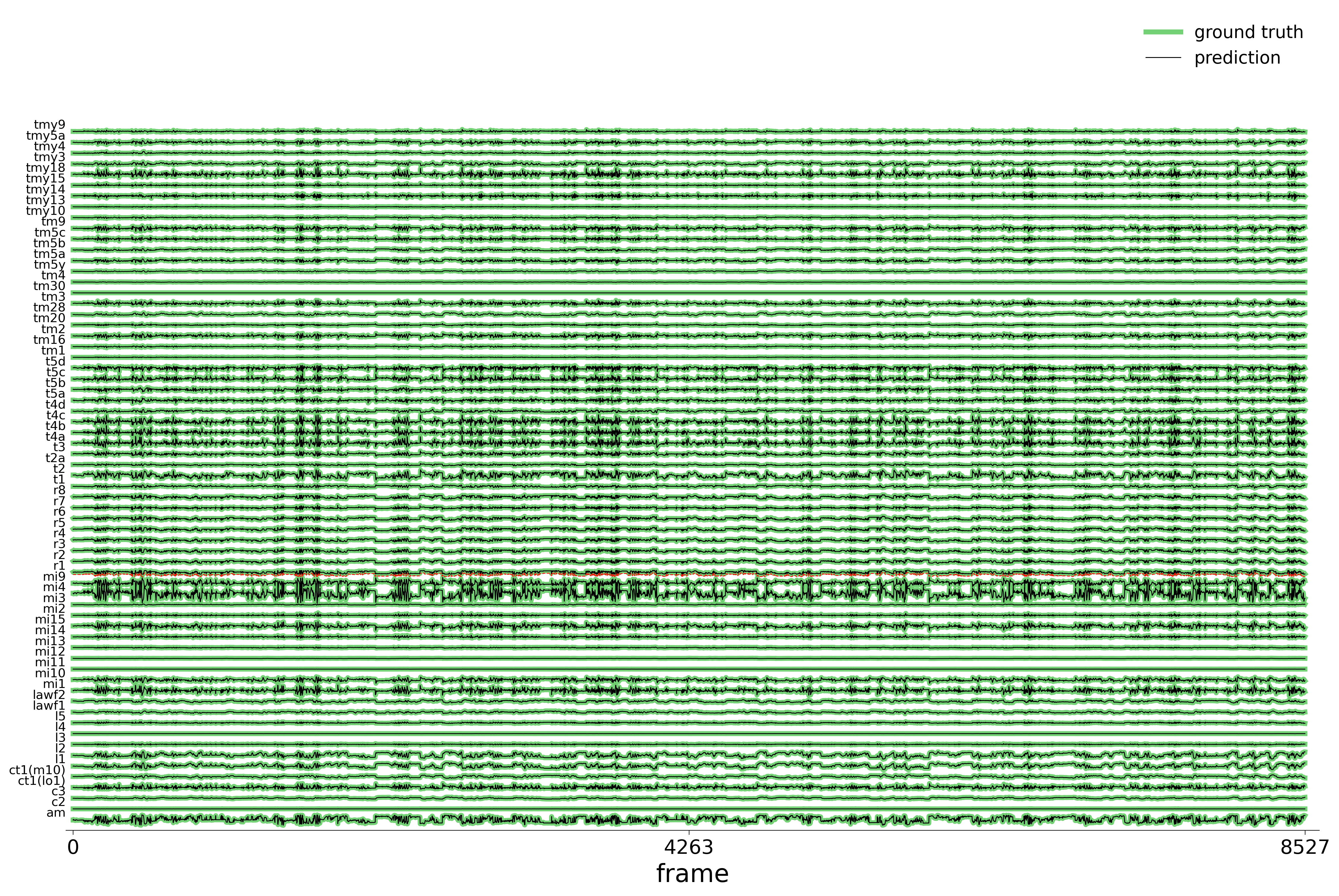
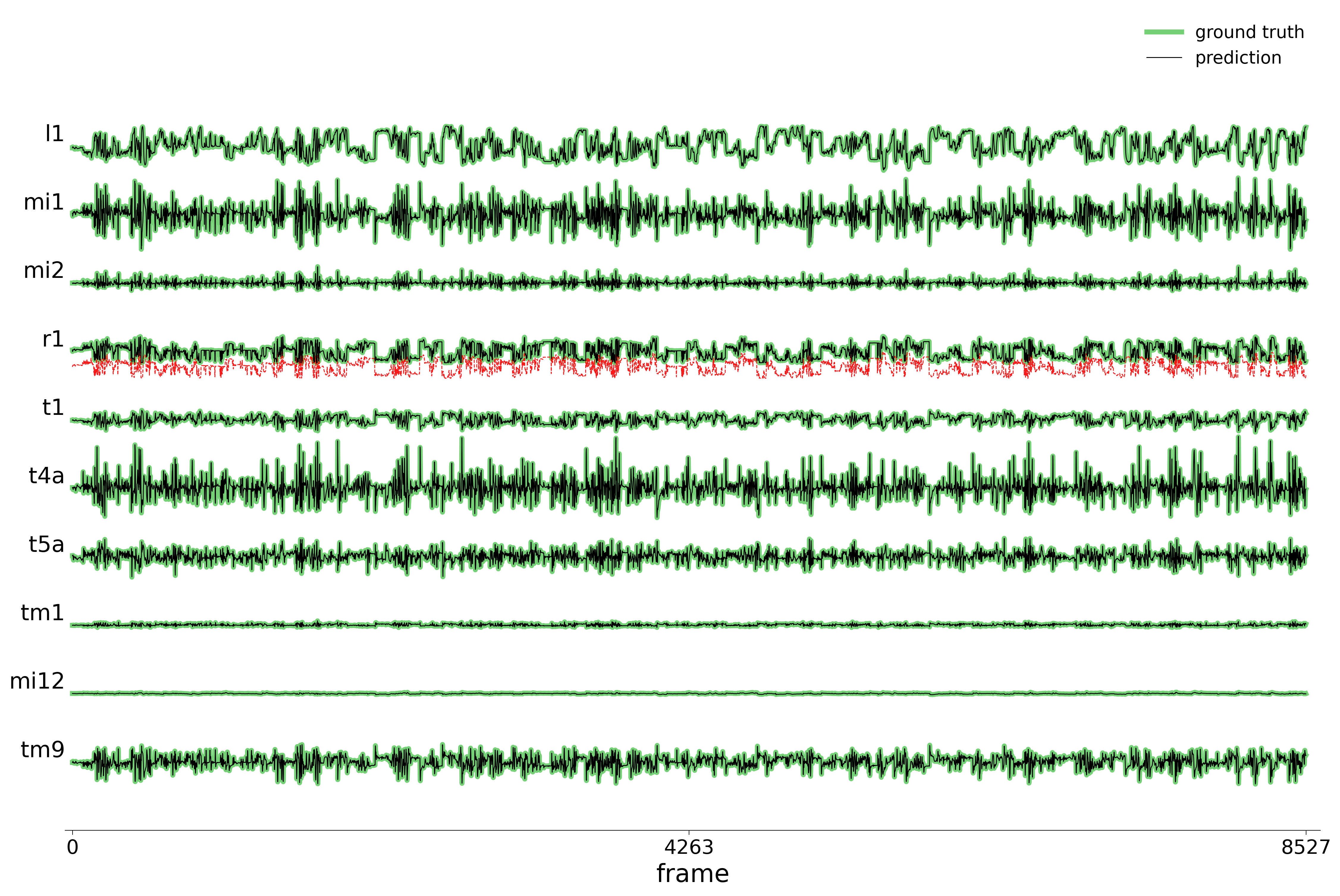
Starting from the initial voltages at \(t{=}0\), the model receives only the external stimulus from the test set (unseen video sequences) and autoregressively integrates its own predicted derivatives to produce the full voltage trajectory. In the plots below, ground-truth traces appear in green and GNN predictions in black. The red trace corresponds to one of the R1–R6 outer photoreceptors, which receive the visual stimulus directly from the compound eye while also integrating excitatory feedback from lamina interneurons (L2, L4, and amacrine cells). The all-types plot displays one representative neuron per cell type (65 traces in total), giving a broad overview of how well the GNN captures the diversity of circuit dynamics across all cell classes. The selected plot zooms into a smaller subset of neurons chosen to highlight fine temporal structure and allow a more detailed comparison between prediction and ground truth.
Noise-free (\(\sigma = 0\))
Low noise (\(\sigma = 0.05\))
High noise (\(\sigma = 0.5\))
Test Metrics
The model was evaluated in two modes: one-step prediction (ground-truth voltages at each frame, predicting \(\widehat{dv}/dt\)) and autoregressive rollout (integrating its own predictions from the first frame, receiving only the external stimulus). The tables below summarize the quantitative evaluation for each noise condition. RMSE measures the average magnitude of prediction errors across all neurons, while Pearson \(r\) captures how well the predicted and ground-truth temporal profiles are correlated on a per-neuron basis (reported as mean \(\pm\) standard deviation over neurons).
One-Step Prediction (test set)
Metric
Noise-free
Noise 0.05
Noise 0.5
RMSE
0.1629 +/- 0.1177
0.2636 +/- 0.2061
0.3742 +/- 0.3029
Pearson r
0.997 +/- 0.018
0.999 +/- 0.002
1.000 +/- 0.000
Autoregressive Rollout (test set)
Metric
Noise-free
Noise 0.05
Noise 0.5
RMSE
0.0085 +/- 0.0064
0.1106 +/- 0.0592
0.8452 +/- 0.3531
Pearson r
0.997 +/- 0.015
0.779 +/- 0.238
0.173 +/- 0.146
Noise-Free Evaluation
A key question is whether models trained on noisy data have learned the underlying deterministic dynamics. To test this, the noisy models (\(\sigma{=}0.05\) and \(\sigma{=}0.5\)) are evaluated on the noise-free test data. If the GNN has correctly identified the noiseless update rule, its rollout on clean data should track the deterministic ground truth closely.
Code
noise_free_config = configs['flyvis_noise_free']noisy_datasets = [ds for ds in datasets if ds[0] !='flyvis_noise_free']for config_name, label in noisy_datasets: config = configs[config_name]print()print(f"--- {label} model on noise-free test data ---") data_test(config, best_model='best', device=device, test_config=noise_free_config)
Rollout: Noisy Models on Noise-Free Data
Low noise (\(\sigma = 0.05\)) model on noise-free data
High noise (\(\sigma = 0.5\)) model on noise-free data
Noise-Free Rollout Metrics
Metric
Noise 0.05
Noise 0.5
RMSE
0.0219 +/- 0.0204
0.0112 +/- 0.0100
Pearson r
0.991 +/- 0.069
0.984 +/- 0.162
Noise and Denoising
When the training data contains process noise (\(\sigma = 0.05\) or \(\sigma = 0.5\)), the stochastic component of the derivatives \(\sigma\,\xi_i(t)\) is, by definition, unpredictable from the current state. A model that minimizes mean-squared error will therefore learn to predict only the deterministic part of \(dv_i/dt\), effectively ignoring the noise. The GNN has in fact learned a noise-free dynamical model: it recovers the deterministic update rule underlying the noisy observations.
The rollout traces and metrics above confirm this interpretation. Models trained on noisy data, when evaluated on noise-free test stimuli, track the clean ground truth with high fidelity. This demonstrates that the GNN implicitly denoises the dynamics. It extracts the systematic circuit computation from stochastic observations without any explicit noise model or denoising objective.
References
[1] J. K. Lappalainen et al., “Connectome-constrained networks predict neural activity across the fly visual system,” Nature, 2024. doi:10.1038/s41586-024-07939-3