config_file = 'signal_N_100_2'
figure_id = 'supp18'
config = ParticleGraphConfig.from_yaml(f'./config/{config_file}.yaml')
device = set_device("auto")Training GNN on signaling
Signaling
GNN Training
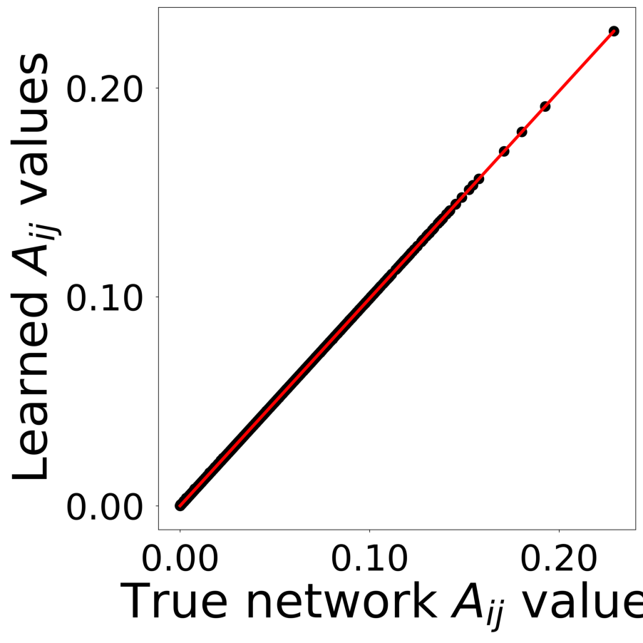
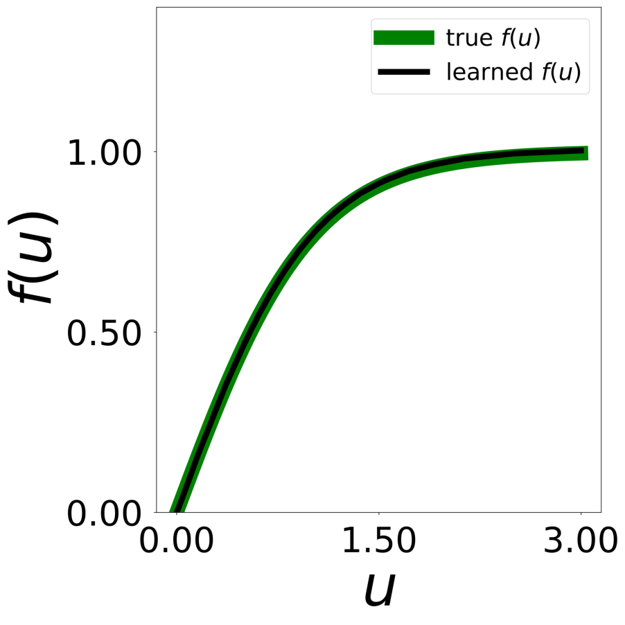
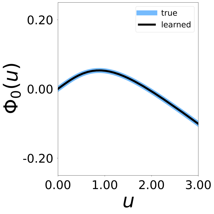
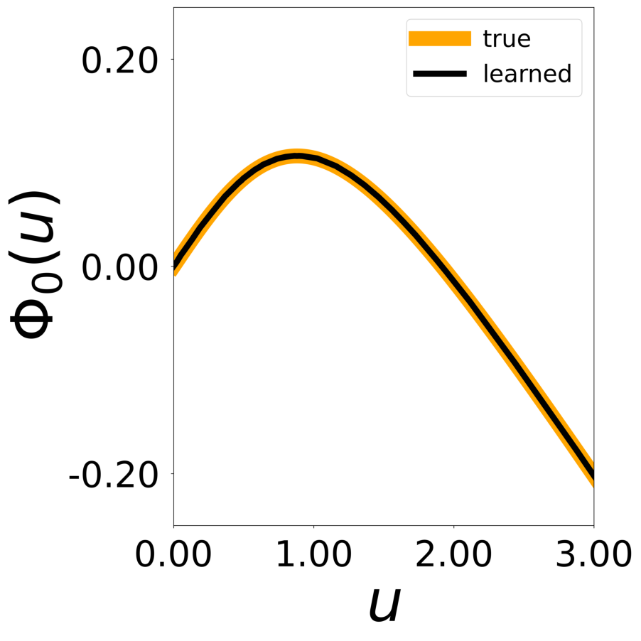
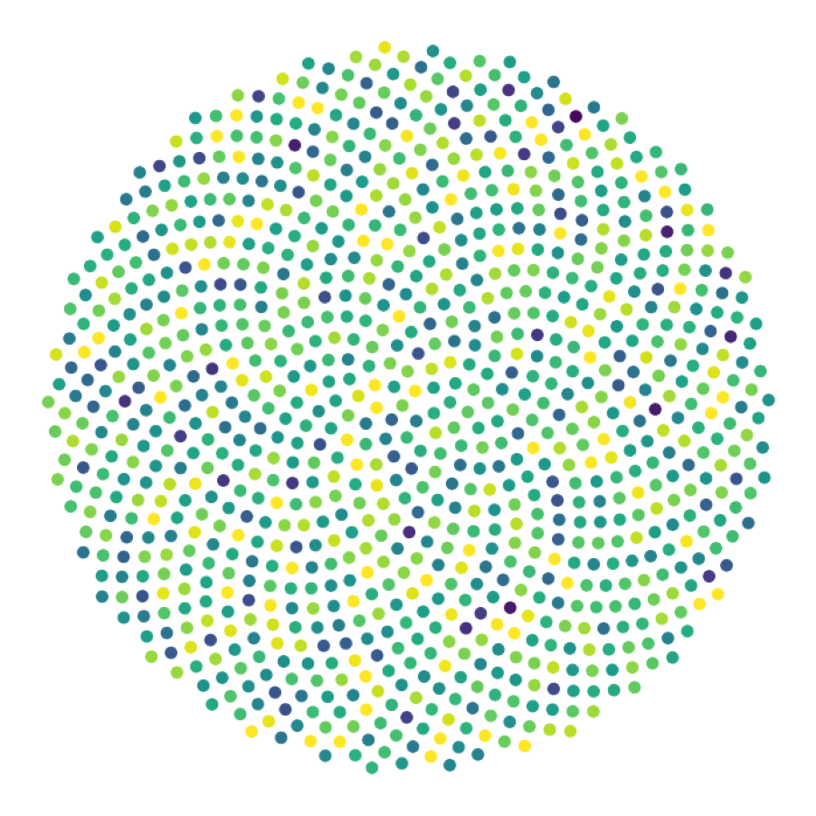
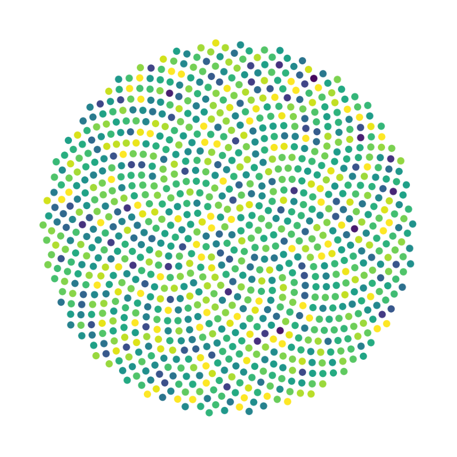
This script generates figures shown in Supplementary Figures 18. A GNN is trained on a signaling network (998 nodes, 17,865 edges). Note 100 of datasets are generated for training.
First, we load the configuration file and set the device.
The following model is used to simulate the signaling network with PyTorch Geometric.
class SignalingNetwork(pyg.nn.MessagePassing):
    """Interaction Network as proposed in this paper:
    https://proceedings.neurips.cc/paper/2016/hash/3147da8ab4a0437c15ef51a5cc7f2dc4-Abstract.html"""

    """

    Inputs
    ----------
    data : a torch_geometric.data object

    Returns
    -------
    pred : float

    """

    def __init__(self, aggr_type=[], p=[], bc_dpos=[]):
        super(SignalingNetwork, self).__init__(aggr=aggr_type)

        self.p = p
        self.bc_dpos = bc_dpos

    def forward(self, data=[], return_all=False):
        x, edge_index, edge_attr = data.x, data.edge_index, data.edge_attr
        edge_index, _ = pyg_utils.remove_self_loops(edge_index)
        particle_type = x[:, 5].long()
        parameters = self.p[particle_type]
        b = parameters[:, 0:1]
        c = parameters[:, 1:2]

        u = x[:, 6:7]

        msg = self.propagate(edge_index, u=u, edge_attr=edge_attr)

        du = -b * u + c * torch.tanh(u) + msg

        if return_all:
            return du, -b * u + c * torch.tanh(u), msg
        else:
            return du

    def message(self, u_j, edge_attr):

        self.activation = torch.tanh(u_j)
        self.u_j = u_j

        return edge_attr[:, None] * torch.tanh(u_j)


def bc_pos(x):
    return torch.remainder(x, 1.0)


def bc_dpos(x):
    return torch.remainder(x - 0.5, 1.0) - 0.5
The data is generated with the above Pytorch Geometric model. If the simulation is too large, you can decrease n_particles (multiple of 2) and n_nodes in “signal_N_100_2.yaml”
p = torch.squeeze(torch.tensor(config.simulation.params))
model = SignalingNetwork(aggr_type=config.graph_model.aggr_type, p=torch.squeeze(p), bc_dpos=bc_dpos)

generate_kwargs = dict(device=device, visualize=True, run_vizualized=0, style='color', alpha=1, erase=True, save=True, step=10)
train_kwargs = dict(device=device, erase=True)
test_kwargs = dict(device=device, visualize=True, style='color', verbose=False, best_model='7', run=0, step=10, save_velocity=True)

data_generate_synaptic(config, model, **generate_kwargs)
Finally, we generate the figures that are shown in Figure 2. The frames of the first six datasets are saved in ‘decomp-gnn/paper_experiments/graphs_data/graphs_signal_N_100_2/Fig/’.


The GNN model (see src/ParticleGraph/models/Signal_Propagation.py) is trained and tested.
Since we ship the trained model with the repository, this step can be skipped if desired.
if not os.path.exists(f'log/try_{config_file}'):
    data_train(config, config_file, **train_kwargs)
During training the plot of the embedding are saved in “paper_experiments/log/try_signal_N_100_2/tmp_training/embedding” The plot of the pairwise interactions are saved in “paper_experiments/log/try_signal_N_100_2/tmp_training/function”
The model that has been trained in the previous step is used to generate the rollouts.
data_test(config, config_file, **test_kwargs)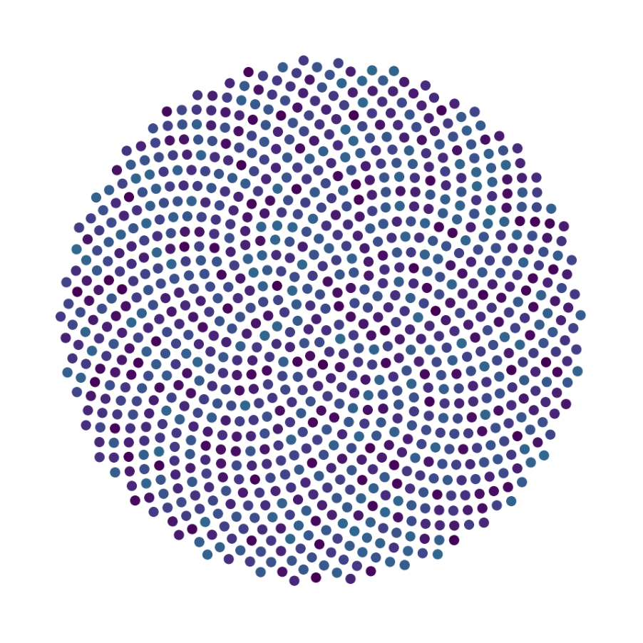


Finally, we generate figures from the post-analysis of the GNN. The results of the GNN post-analysis are saved into ‘decomp-gnn/paper_experiments/log/try_signal_N_100_2/results’.
config_list, epoch_list = get_figures(figure_id, device=device)