Training GNN on reaction-diffusion (rock-paper-scissors)

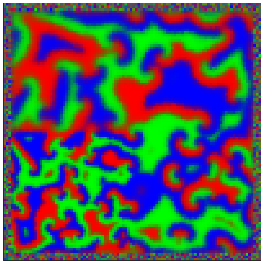
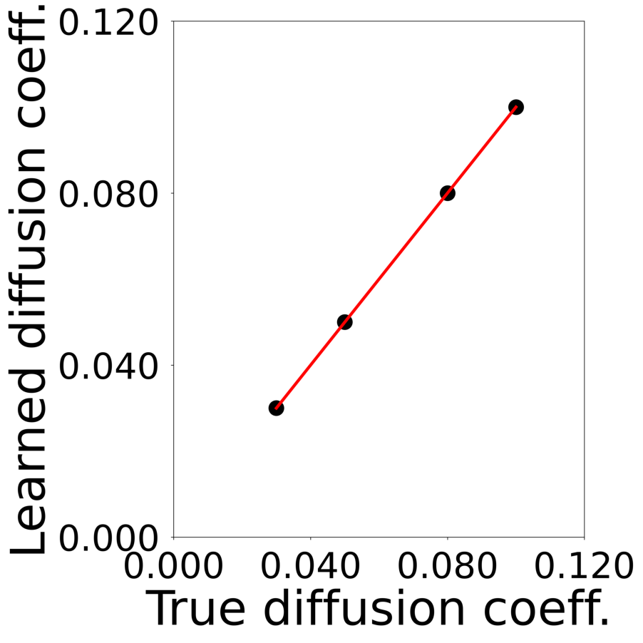
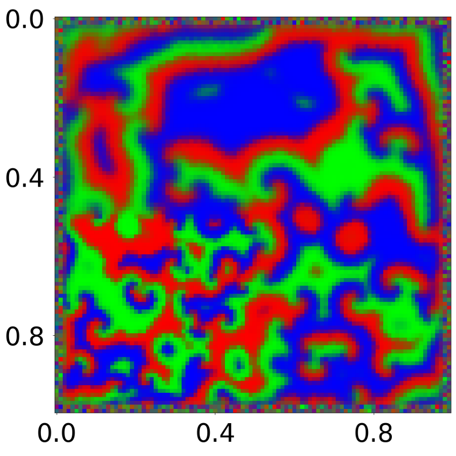
This script generates Supplementary Figure 17. It showcases a Graph Neural Network (GNN) learning the dynamics of a reaction-diffusion system. The training simulation involves 1E4 mesh nodes observed over 4E3 frames. Node interactions follow rock-paper-scissors rules with different diffusion coefficients.

First, we load the configuration file and set the device.

config_file = 'RD_RPS'
figure_id = 'supp17'
config = ParticleGraphConfig.from_yaml(f'./config/{config_file}.yaml')
device = set_device("auto")

The following model is used to simulate the ‘rock-paper-scissor’ model with PyTorch Geometric.

class RDModel(pyg.nn.MessagePassing):
    """Interaction Network as proposed in this paper:
    https://proceedings.neurips.cc/paper/2016/hash/3147da8ab4a0437c15ef51a5cc7f2dc4-Abstract.html"""

    """
    Compute the reaction diffusion according to the rock paper scissor model.

    Inputs
    ----------
    data : a torch_geometric.data object
    Note the Laplacian coeeficients are in data.edge_attr

    Returns
    -------
    increment : float
        the first derivative of three scalar fields u, v and w

    """

    def __init__(self, aggr_type=[], bc_dpos=[], coeff = []):
        super(RDModel, self).__init__(aggr='add')  # "mean" aggregation.

        self.bc_dpos = bc_dpos
        self.coeff = coeff
        self.a = 0.6

    def forward(self, data):
        x, edge_index, edge_attr = data.x, data.edge_index, data.edge_attr

        c = self.coeff

        uvw = data.x[:, 6:9]
        laplace_uvw = c * self.propagate(data.edge_index, uvw=uvw, discrete_laplacian=data.edge_attr)
        p = torch.sum(uvw, axis=1)

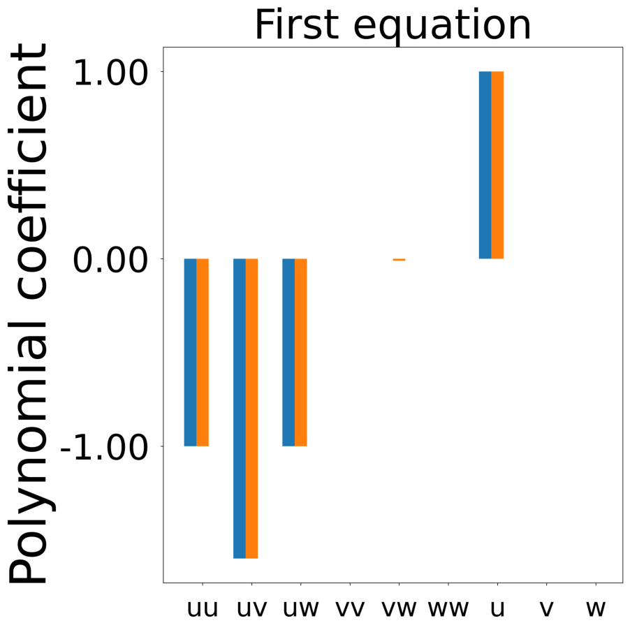
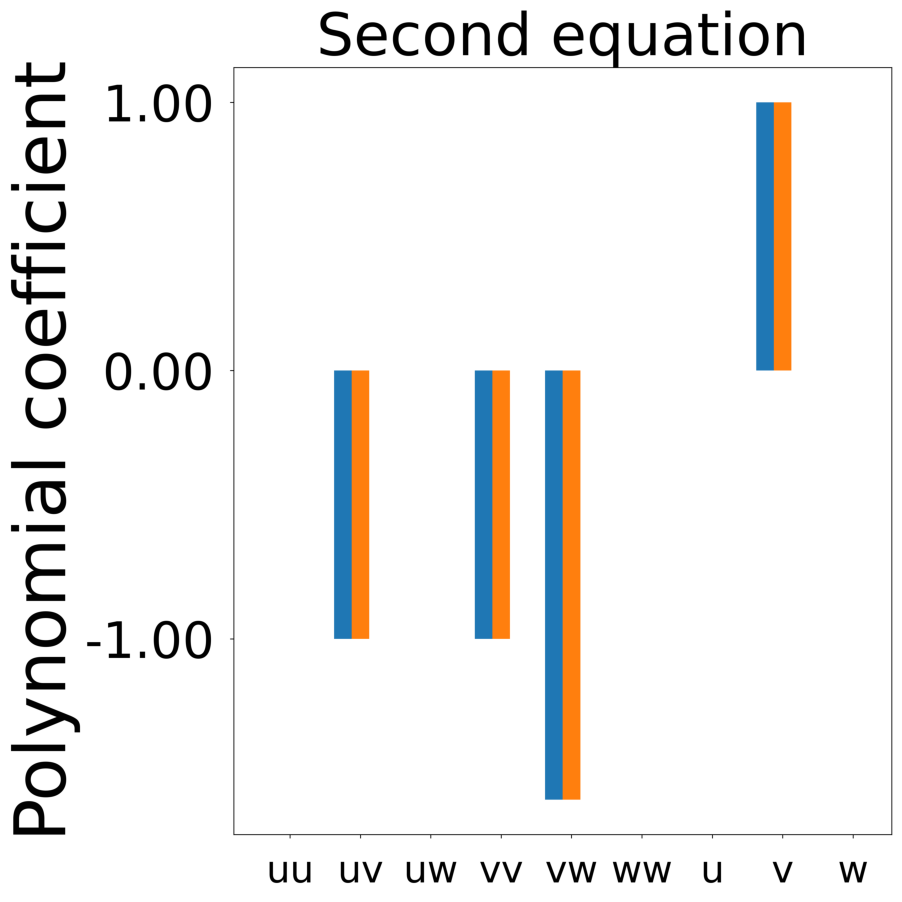
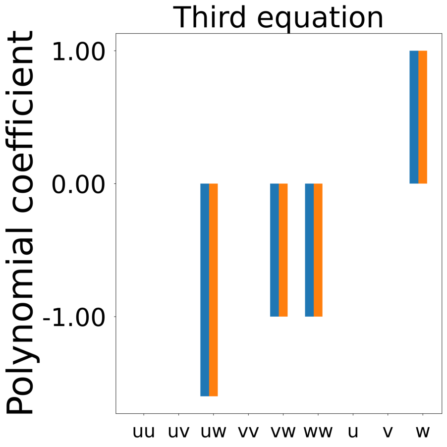
        d_uvw = laplace_uvw + uvw * (1 - p[:, None] - self.a * uvw[:, [1, 2, 0]])
        # This is equivalent to the nonlinear reaction diffusion equation:
        #   du = D * laplace_u + u * (1 - p - a * v)
        #   dv = D * laplace_v + v * (1 - p - a * w)
        #   dw = D * laplace_w + w * (1 - p - a * u)

        return d_uvw

    def message(self, uvw_j, discrete_laplacian):
        return discrete_laplacian[:, None] * uvw_j


def bc_pos(x):
    return torch.remainder(x, 1.0)


def bc_dpos(x):
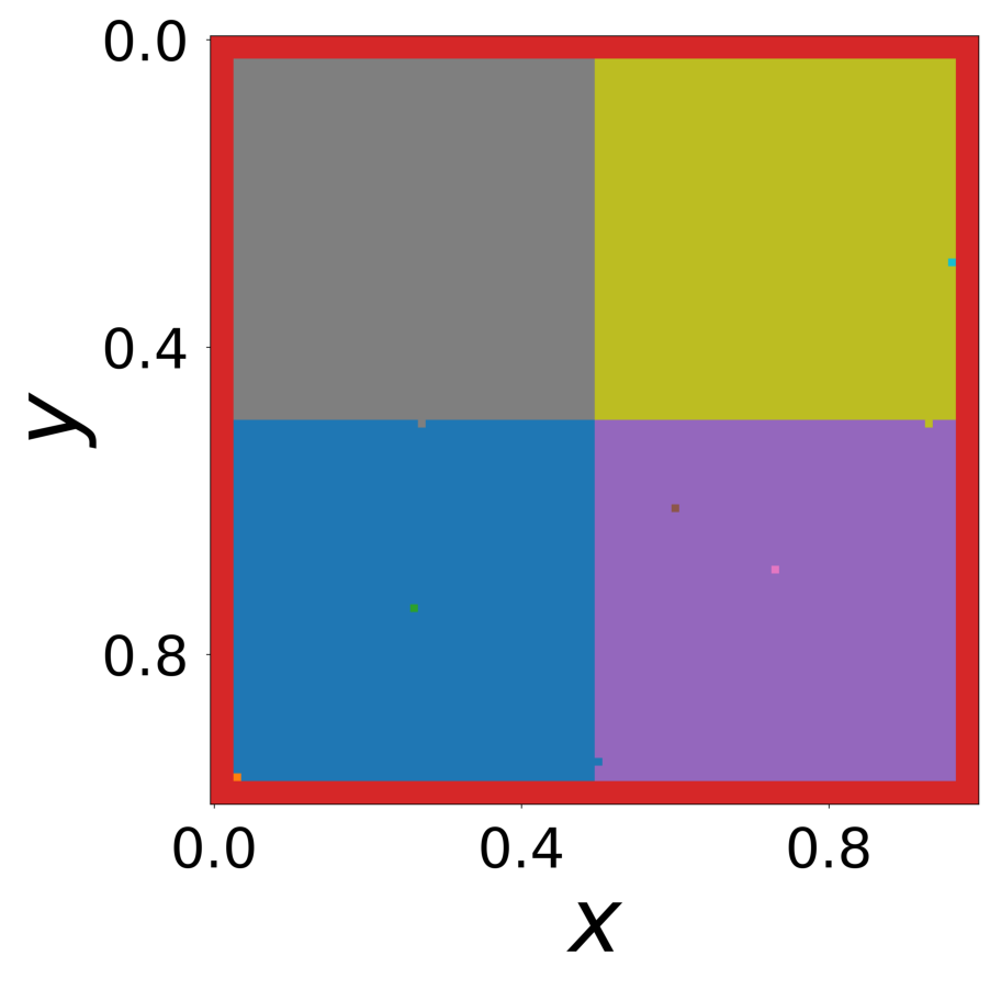
    return torch.remainder(x - 0.5, 1.0) - 0.5

The coefficients of diffusion are loaded from a tif file specified in the config yaml file and the data is generated.

Vizualizations of the reaction diffusion can be found in “decomp-gnn/paper_experiments/graphs_data/RD_RPS/”

If the simulation is too large, you can decrease n_particles and n_nodes in “RD_RPS.yaml”.

model = RDModel(
    aggr_type='add',
    bc_dpos=bc_dpos)

generate_kwargs = dict(device=device, visualize=True, run_vizualized=0, style='color', erase=False, save=True, step=50)
train_kwargs = dict(device=device, erase=True)
test_kwargs = dict(device=device, visualize=True, style='color', verbose=False, best_model='20', run=0, step=20)

data_generate_mesh(config, model , **generate_kwargs)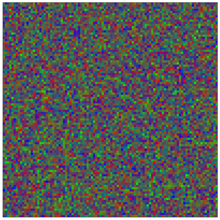

Initial configuration of the simulation. There are 1E4 nodes. The colors indicate the node vector values.

Frame 3750 out of 4000

The GNN model (see src/ParticleGraph/models/Mesh_RPS.py) is optimized using the ‘rock-paper-scissor’ data.

Since we ship the trained model with the repository, this step can be skipped if desired.

if not os.path.exists(f'log/try_{config_file}'):
    data_train(config, config_file, **train_kwargs)

The model that has been trained in the previous step is used to generate the rollouts. The rollout visualization can be found in paper_experiments/log/try_RD_RPS/tmp_recons.

data_test(config, config_file, **test_kwargs)

Finally, we generate the figures that are shown in Supplementary Figure 17. The results of the GNN post-analysis are saved into ‘decomp-gnn/paper_experiments/log/try_RD_RPS/results’.

config_list, epoch_list = get_figures(figure_id, device=device)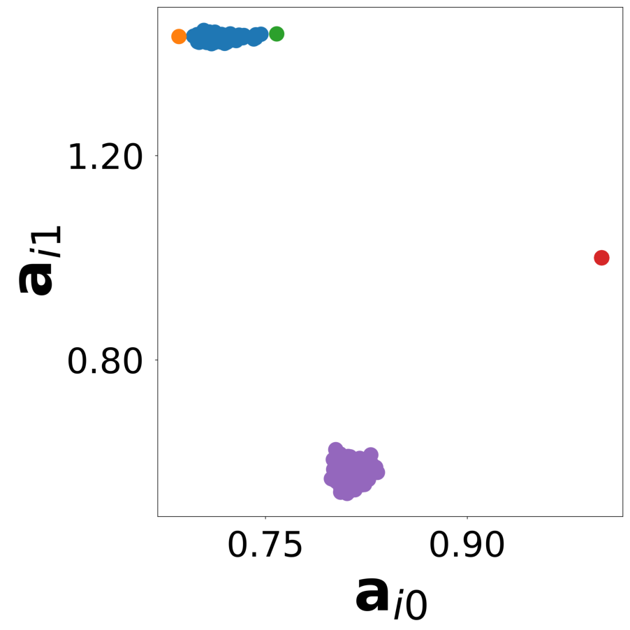

Learned latent vectors (x1E4)

Learned map of of node type

Comparison between true and learned coefficients of diffusion

Comparison between true (blue) and learned (orange) polynomial coefficients of the first governing equation

Comparison between true (blue) and learned (orange) polynomial coefficients of the second governing equation

Comparison between true (blue) and learned (orange) polynomial coefficients of the third gooverning equation

GNN rollout inference at frame 3980

All frames can be found in “decomp-gnn/paper_experiments/log/try_RD_RPS/tmp_recons/”