Training GNN on attraction-repulsion (hidden field)

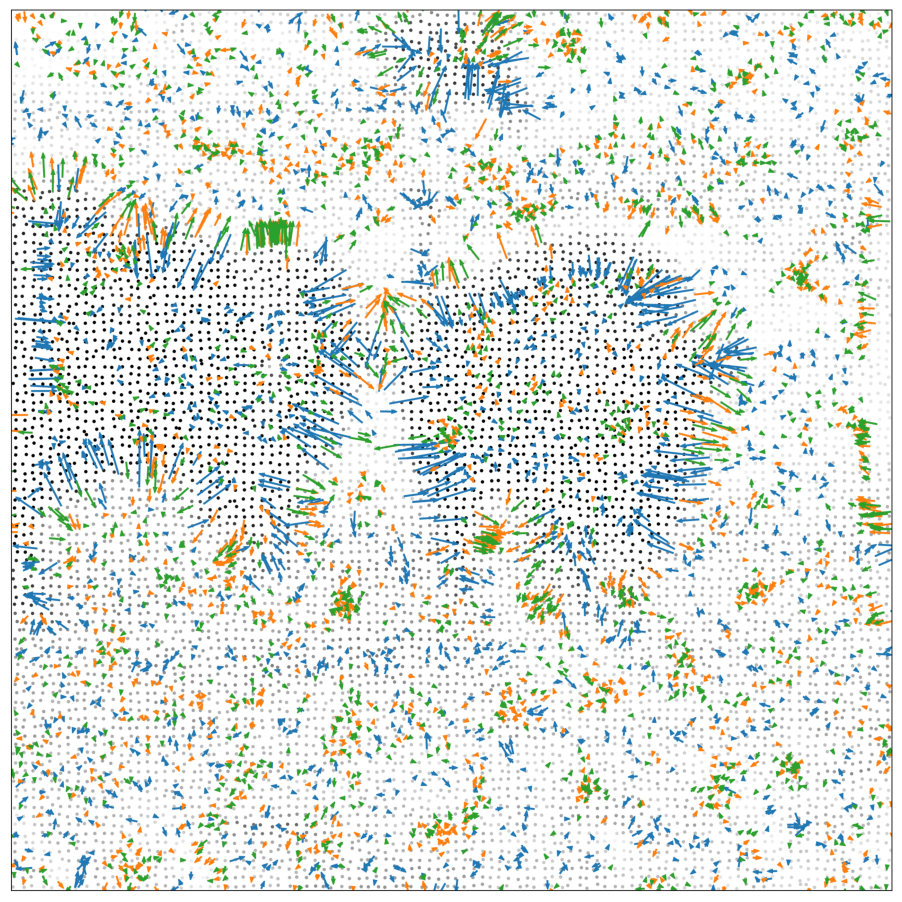
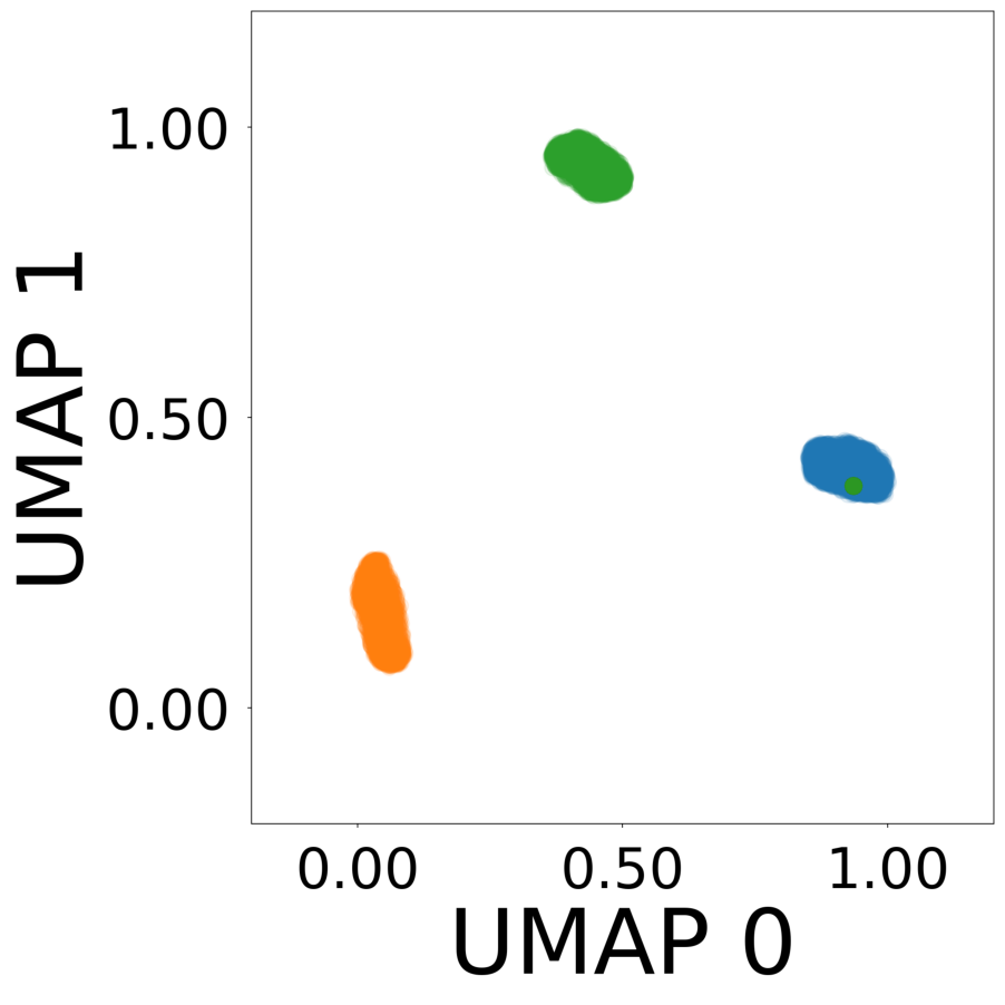
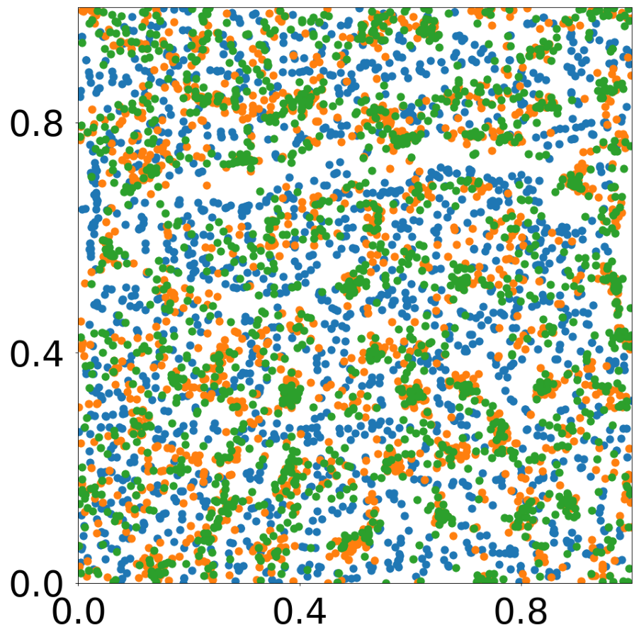
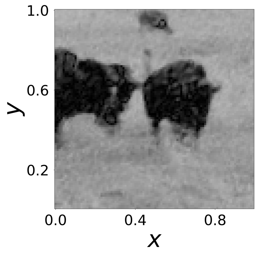
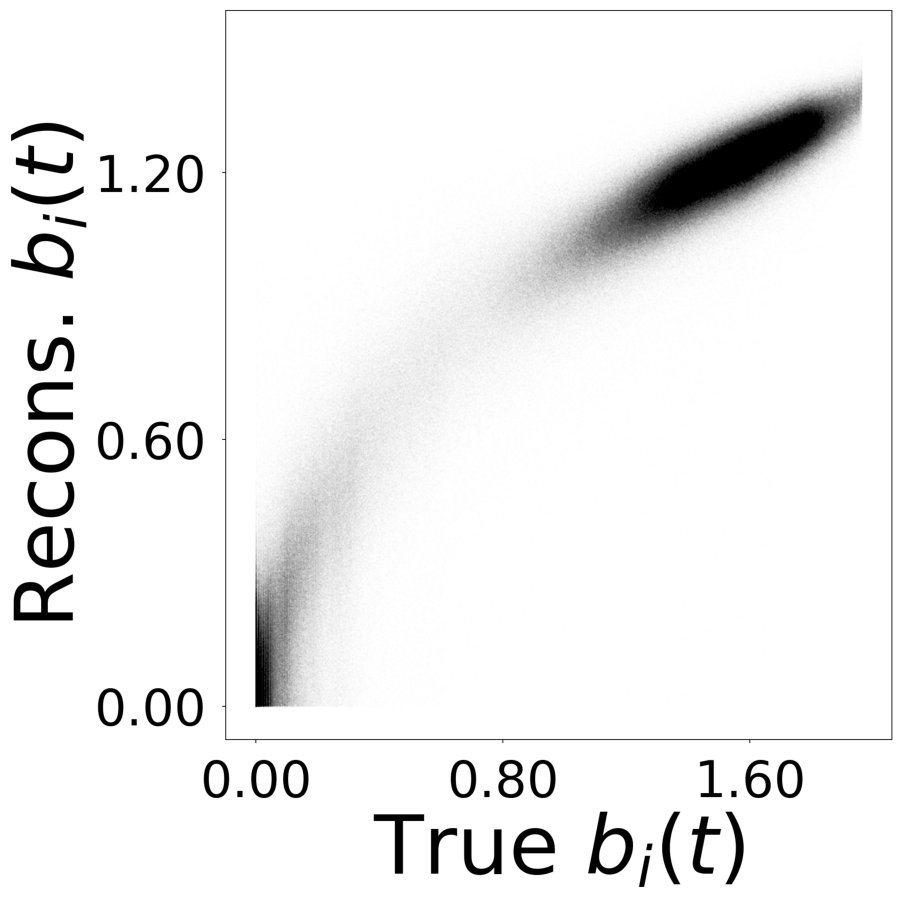
This script creates figure of paper’s Figure 4. A GNN learns the motion rules of an attraction-repulsion system. The simulation used to train the GNN consists of 4800 particles of three different types. The particles interact with each other according to three different attraction-repulsion laws. The particle interact also with a hidden dynamical field.

First, we load the configuration file and set the device.

config_file = 'arbitrary_3_field_video'
figure_id = '4'
config = ParticleGraphConfig.from_yaml(f'./config/{config_file}.yaml')
device = set_device("auto")

The following model is used to simulate the attraction-repulsion system with PyTorch Geometric.

class ParticleField(pyg.nn.MessagePassing):
    """Interaction Network as proposed in this paper:
    https://proceedings.neurips.cc/paper/2016/hash/3147da8ab4a0437c15ef51a5cc7f2dc4-Abstract.html"""

    """
    Compute the speed of particles as a function of their relative position according to an attraction-repulsion law.
    The latter is defined by four parameters p = (p1, p2, p3, p4) and a parameter sigma.

    See https://github.com/gpeyre/numerical-tours/blob/master/python/ml_10_particle_system.ipynb

    Inputs
    ----------
    data : a torch_geometric.data object

    Returns
    -------
    pred : float
        the speed of the particles (dimension 2)
    """

    def __init__(self, aggr_type=[], p=[], sigma=[], bc_dpos=[], dimension=2):
        super(ParticleField, self).__init__(aggr=aggr_type)  # "mean" aggregation.

        self.p = p
        self.sigma = sigma
        self.bc_dpos = bc_dpos
        self.dimension = dimension

    def forward(self, data=[], has_field=False):
        x, edge_index = data.x, data.edge_index

        if has_field:
            field = x[:,6:7]
        else:
            field = torch.ones_like(x[:,0:1])

        edge_index, _ = pyg_utils.remove_self_loops(edge_index)
        particle_type = to_numpy(x[:, 1 + 2*self.dimension])
        parameters = self.p[particle_type,:]
        d_pos = self.propagate(edge_index, pos=x[:, 1:self.dimension+1], parameters=parameters, field=field)
        return d_pos

    def message(self, pos_i, pos_j, parameters_i, field_j):

        distance_squared = torch.sum(self.bc_dpos(pos_j - pos_i) ** 2, axis=1)  # squared distance
        f = (parameters_i[:, 0] * torch.exp(-distance_squared ** parameters_i[:, 1] / (2 * self.sigma ** 2))
               - parameters_i[:, 2] * torch.exp(-distance_squared ** parameters_i[:, 3] / (2 * self.sigma ** 2)))
        d_pos = f[:, None] * self.bc_dpos(pos_j - pos_i) * field_j

        return d_pos

    def psi(self, r, p):
        return r * (p[0] * torch.exp(-r ** (2 * p[1]) / (2 * self.sigma ** 2))
                    - p[2] * torch.exp(-r ** (2 * p[3]) / (2 * self.sigma ** 2)))


def bc_pos(x):
    return torch.remainder(x, 1.0)


def bc_dpos(x):
    return torch.remainder(x - 0.5, 1.0) - 0.5

The training data is generated with the above Pytorch Geometric model

Vizualizations of the particle motions can be found in “decomp-gnn/paper_experiments/graphs_data/graphs_arbitrary_3_field_video/”

If the simulation is too large, you can decrease n_particles (multiple of 3) and n_nodes in “arbitrary_3_field_video.yaml”

p = torch.squeeze(torch.tensor(config.simulation.params))
sigma = config.simulation.sigma
model = ParticleField(
    aggr_type=config.graph_model.aggr_type,
    p=p,
    sigma=sigma,
    bc_dpos=bc_dpos,
    dimension=config.simulation.dimension
)

generate_kwargs = dict(device=device, visualize=True, run_vizualized=0, style='color', alpha=1, erase=True, save=True, step=20)
train_kwargs = dict(device=device, erase=True)
test_kwargs = dict(device=device, visualize=True, style='color', verbose=False, best_model='20', run=0, step=20, save_velocity=True)

data_generate_particle_field(config, model, bc_pos, bc_dpos, **generate_kwargs)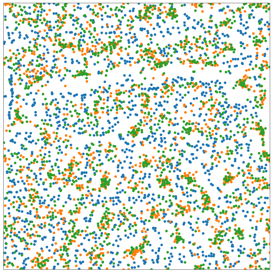

Frame 100. The orange, blue, and green particles represent the three different particle types.

Frame 100. The arrows shows the influence of the hidden field on the particles velocity field.

The GNN model (see src/ParticleGraph/models/Interaction_Particle.py) is trained and tested.

Since we ship the trained model with the repository, this step can be skipped if desired.

During training the plots of the embedding are saved in “paper_experiments/log/try_arbitrary_3_field_video/tmp_training/embedding”. The plots of the interaction functions are saved in “function” and the hidden field in “field”.

if not os.path.exists(f'log/try_{config_file}'):
    data_train(config, config_file, **train_kwargs)

The model that has been trained in the previous step is used to generate the rollouts.

data_test(config, config_file, **test_kwargs)

Finally, we generate the figures that are shown in Figure 4. The results of the GNN post-analysis are saved into ‘decomp-gnn/paper_experiments/log/try_arbitrary_3_field_video/results’.

config_list, epoch_list = get_figures(figure_id, device=device)

Learned latent vectors (x4800)

Learned interaction functions (x3)

UMAP projection of the learned interaction functions (x3)

GNN rollout inference at frame 100

Reconstructed field at frame 100

Comparison betwween true and learned hidden field values

All frames can be found in “decomp-gnn/paper_experiments/log/try_arbitrary_3_field_video/tmp_recons/”