Training GNN on attraction-repulsion (asymmetric, 3 particle types)

Particles

GNN Training

Author

Cédric Allier, Michael Innerberger, Stephan Saalfeld

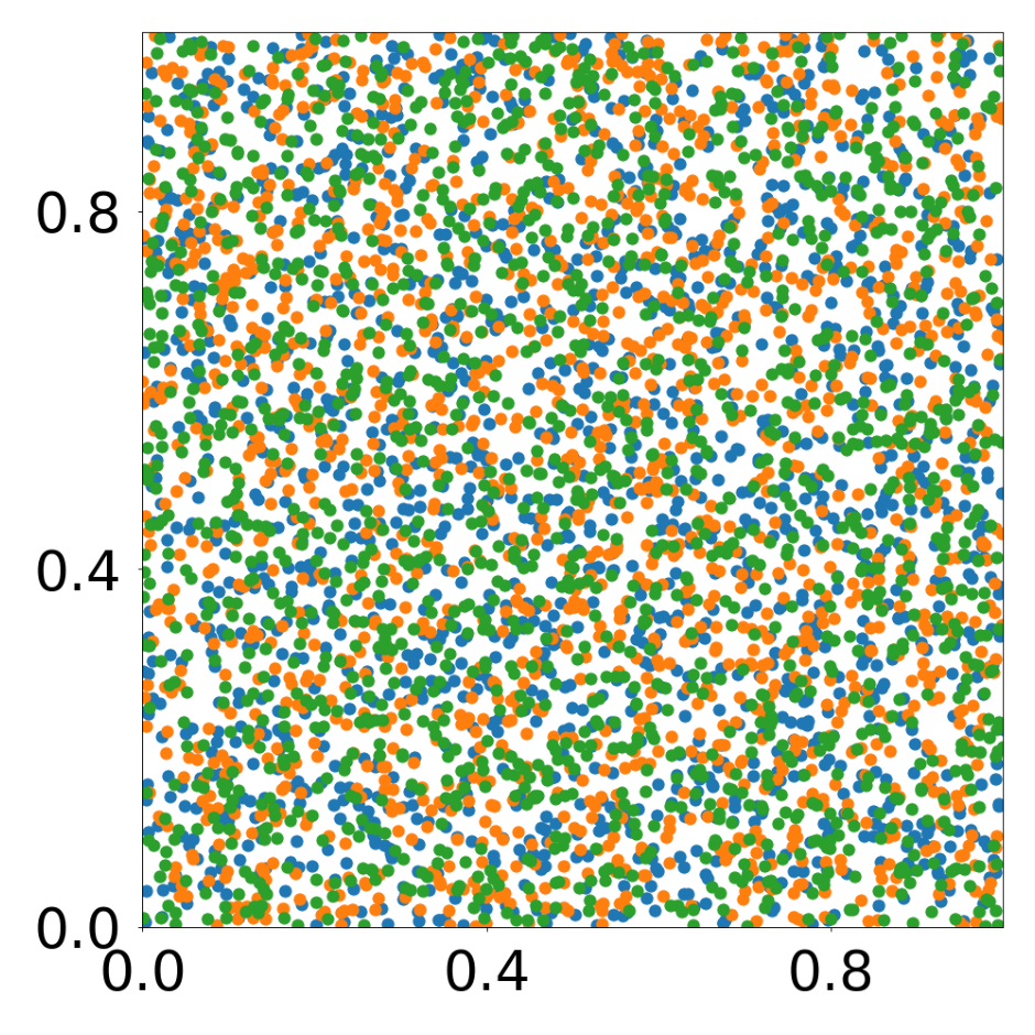
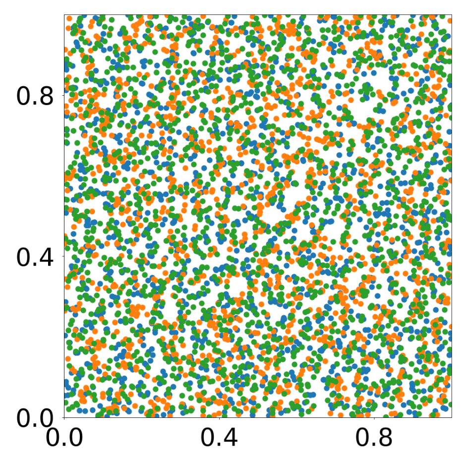
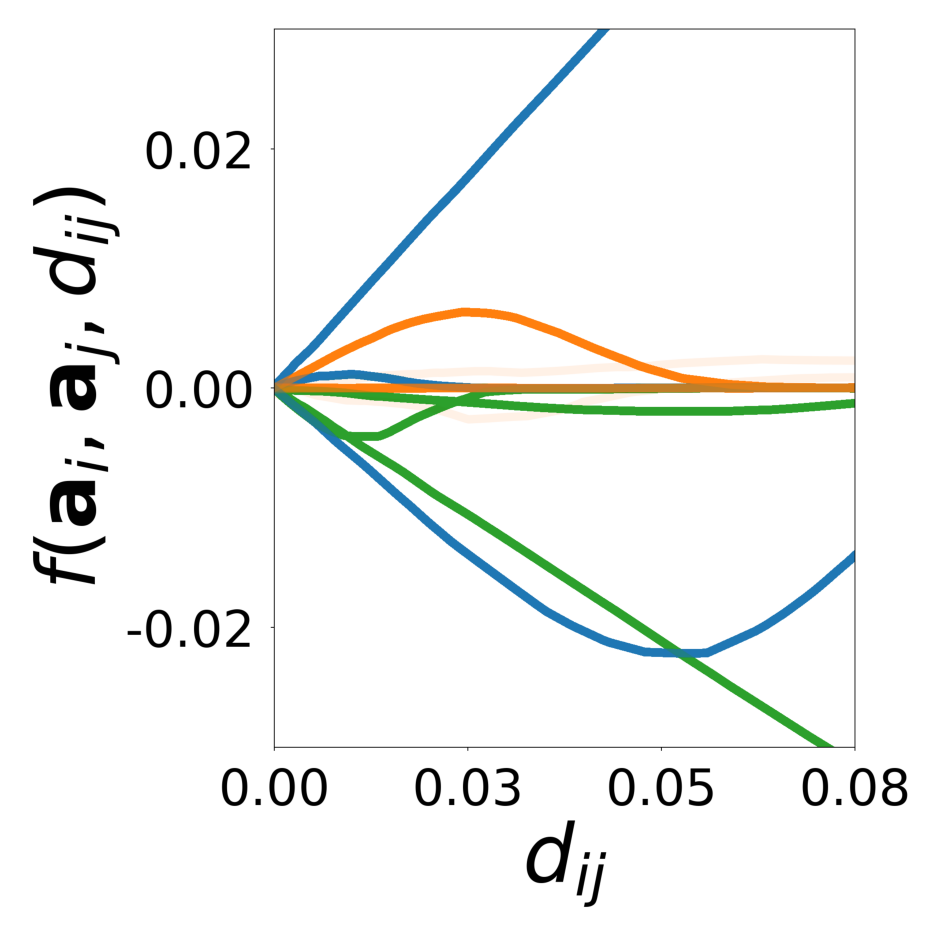
This script creates the second column of paper’s Figure 3. A GNN learns the motion rules of an asymmetric attraction-repulsion system The simulation used to train the GNN consists of 4800 particles of three different types. The particles interact with each other according to 9 different attraction-repulsion laws. The interaction functions asymmetrically depend on the types of both particles.

First, we load the configuration file and set the device.

config_file = 'arbitrary_3_3'
figure_id = '3_2'
config = ParticleGraphConfig.from_yaml(f'./config/{config_file}.yaml')
device = set_device("auto")

The following model is used to simulate the attraction-repulsion system with PyTorch Geometric.

class AttractionRepulsionModel(pyg.nn.MessagePassing):
    """
    Compute the speed of particles as a function of their relative position according to an attraction-repulsion law.
    The latter is defined by four parameters p = (p1, p2, p3, p4) and a parameter sigma.

    See https://github.com/gpeyre/numerical-tours/blob/master/python/ml_10_particle_system.ipynb
    """

    def __init__(self, p=[], sigma=[], bc_dpos=[]):
        super(AttractionRepulsionModel, self).__init__(aggr='mean')  # "mean" aggregation.

        self.p = p
        self.sigma = sigma
        self.bc_dpos = bc_dpos

    def forward(self, data):
        x, edge_index = data.x, data.edge_index
        edge_index, _ = pyg_utils.remove_self_loops(edge_index)
        particle_type = x[:, 5:6]
        d_pos = self.propagate(edge_index, pos=x[:, 1:3], particle_type=particle_type)
        return d_pos

    def message(self, pos_i, pos_j, particle_type_i, particle_type_j):
        distance_squared = torch.sum(self.bc_dpos(pos_j - pos_i) ** 2, axis=1)  # squared distance
        parameters = self.p[to_numpy(particle_type_i), to_numpy(particle_type_j), :].squeeze()

        psi = (parameters[:, 0] * torch.exp(-distance_squared ** parameters[:, 1] / (2 * self.sigma ** 2))
               - parameters[:, 2] * torch.exp(-distance_squared ** parameters[:, 3] / (2 * self.sigma ** 2)))
        d_pos = psi[:, None] * self.bc_dpos(pos_j - pos_i)
        return d_pos

    def psi(self, r, p):
        return r * (p[0] * torch.exp(-r ** (2 * p[1]) / (2 * self.sigma ** 2))
                    - p[2] * torch.exp(-r ** (2 * p[3]) / (2 * self.sigma ** 2)))


def bc_pos(x):
    return torch.remainder(x, 1.0)


def bc_dpos(x):
    return torch.remainder(x - 0.5, 1.0) - 0.5

The training data is generated with the above Pytorch Geometric model

p = torch.squeeze(torch.tensor(config.simulation.params))
sigma = config.simulation.sigma
model = AttractionRepulsionModel(
    p=p,
    sigma=sigma,
    bc_dpos=bc_dpos,
)

generate_kwargs = dict(device=device, visualize=True, run_vizualized=0, style='color', alpha=1, erase=True, save=True, step=10)
train_kwargs = dict(device=device, erase=True)
test_kwargs = dict(device=device, visualize=True, style='color', verbose=False, best_model='20', run=0, step=1, save_velocity=True)

data_generate_particles(config, model, bc_pos, bc_dpos, **generate_kwargs)

The GNN model (see src/ParticleGraph/models/Interaction_Particle.py) is trained and tested.

Since we ship the trained model with the repository, this step can be skipped if desired.

if not os.path.exists(f'log/try_{config_file}'):
    data_train(config, config_file, **train_kwargs)

The model that has been trained in the previous step is used to generate the rollouts. The rollout visualization can be found in paper_experiments/log/try_arbitrary_3_3/tmp_recons.

data_test(config, config_file, **test_kwargs)

Finally, we generate the figures that are shown in Figure 3.

config_list, epoch_list = get_figures(figure_id, device=device)

Initial configuration of the test training dataset. There are 4800 particles. The orange, blue, and green particles represent the three different particle types.