config_file = 'RD_RPS'
config = ParticleGraphConfig.from_yaml(f'./config/{config_file}.yaml')
device = set_device("auto")Reaction-diffusion propagation with different diffusion coefficients
Mesh
Simulation
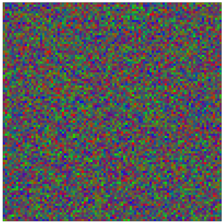
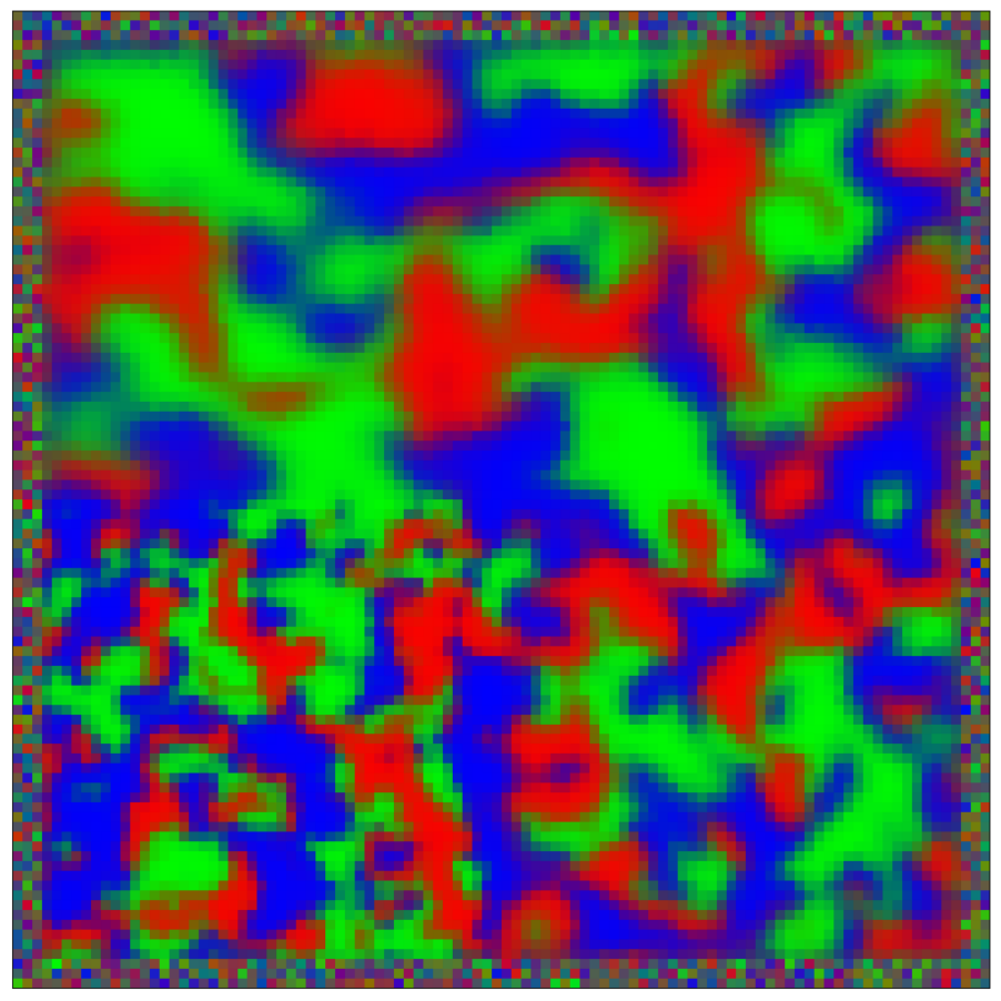
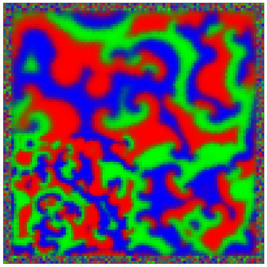
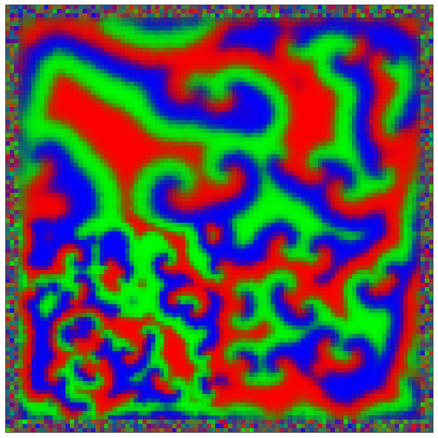
This script creates the sixth column of paper’s Figure 2. Simulation of reaction-diffusion over a mesh of 1E4 nodes with variable propagation-coefficients.
First, we load the configuration file and set the device.
The following model is used to simulate the reaction_diffusion propagation with PyTorch Geometric.
class RDModel(pyg.nn.MessagePassing):
    """Interaction Network as proposed in this paper:
    https://proceedings.neurips.cc/paper/2016/hash/3147da8ab4a0437c15ef51a5cc7f2dc4-Abstract.html"""

    """
    Compute the reaction diffusion according to the rock paper scissor model.

    Inputs
    ----------
    data : a torch_geometric.data object
    Note the Laplacian coeeficients are in data.edge_attr

    Returns
    -------
    increment : float
        the first derivative of three scalar fields u, v and w

    """

    def __init__(self, aggr_type=[], bc_dpos=[], coeff = []):
        super(RDModel, self).__init__(aggr='add')  # "mean" aggregation.

        self.bc_dpos = bc_dpos
        self.coeff = coeff
        self.a = 0.6

    def forward(self, data):
        x, edge_index, edge_attr = data.x, data.edge_index, data.edge_attr

        c = self.coeff

        uvw = data.x[:, 6:9]
        laplace_uvw = c * self.propagate(data.edge_index, uvw=uvw, discrete_laplacian=data.edge_attr)
        p = torch.sum(uvw, axis=1)

        d_uvw = laplace_uvw + uvw * (1 - p[:, None] - self.a * uvw[:, [1, 2, 0]])
        # This is equivalent to the nonlinear reaction diffusion equation:
        #   du = c * laplace_u + u * (1 - p - a * v)
        #   dv = c * laplace_v + v * (1 - p - a * w)
        #   dw = c * laplace_w + w * (1 - p - a * u)

        return d_uvw

    def message(self, uvw_j, discrete_laplacian):
        return discrete_laplacian[:, None] * uvw_j

def bc_pos(x):
    return torch.remainder(x, 1.0)


def bc_dpos(x):
    return torch.remainder(x - 0.5, 1.0) - 0.5
The data is generated with the above Pytorch Geometric model. Note two datasets are generated, one for training and one for validation. If the simulation is too large, you can decrease n_particles (multiple of 5) and n_nodes in “RD_RPS.yaml”
model = RDModel(aggr_type=config.graph_model.aggr_type, bc_dpos=bc_dpos)

generate_kwargs = dict(device=device, visualize=True, run_vizualized=0, style='color', erase=False, save=True, step=10)
train_kwargs = dict(device=device, erase=True)
test_kwargs = dict(device=device, visualize=True, style='color', verbose=False, best_model='20', run=0, step=1, save_velocity=True)

data_generate_mesh(config, model , **generate_kwargs)
Finally, we generate the figures that are shown in Figure 2. All frames are saved in ‘decomp-gnn/paper_experiments/graphs_data/graphs_RD_RPS/Fig/’.