config_file = 'Coulomb_3_256'
config = ParticleGraphConfig.from_yaml(f'./config/{config_file}.yaml')
device = set_device("auto")Coulomb-like system with different particle charges
Particles
Simulation
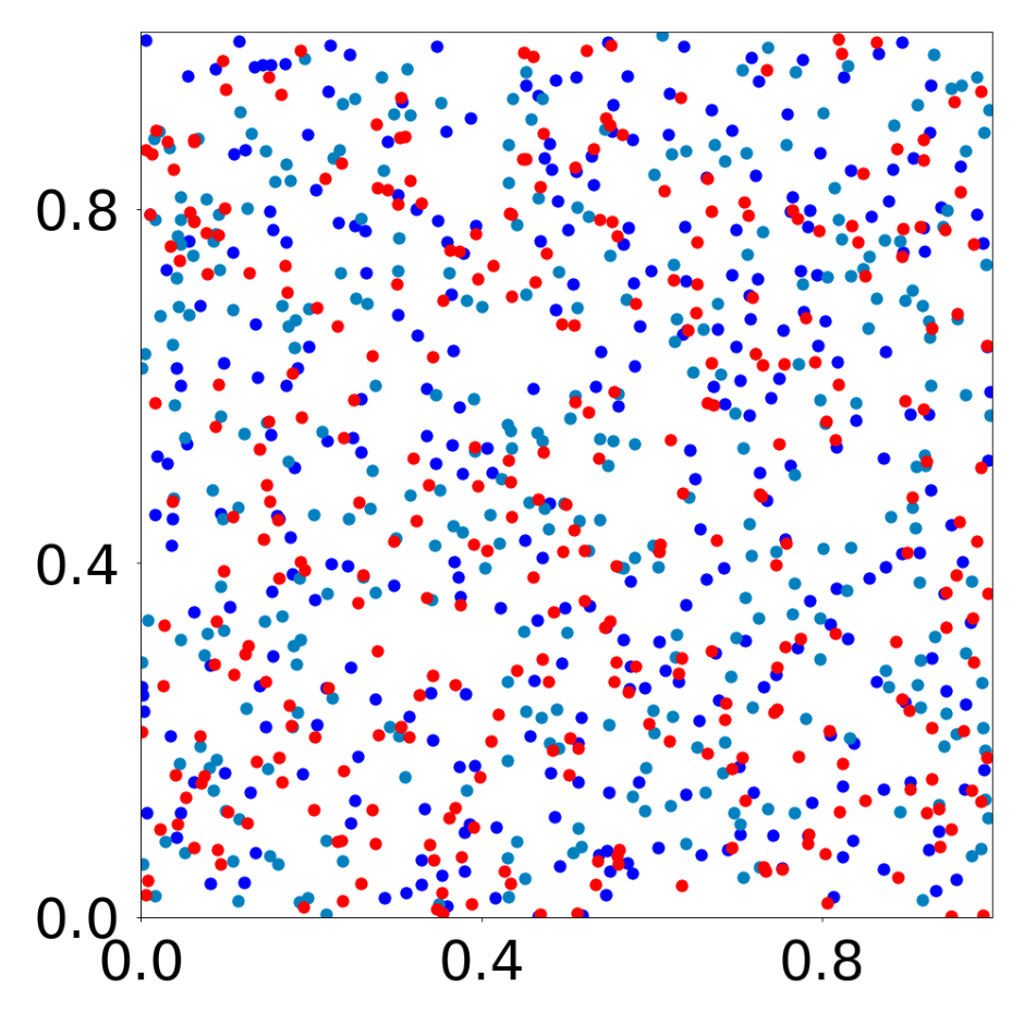
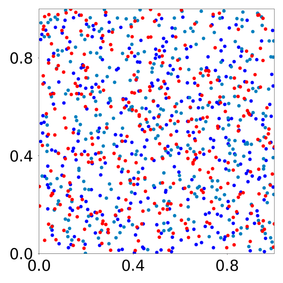
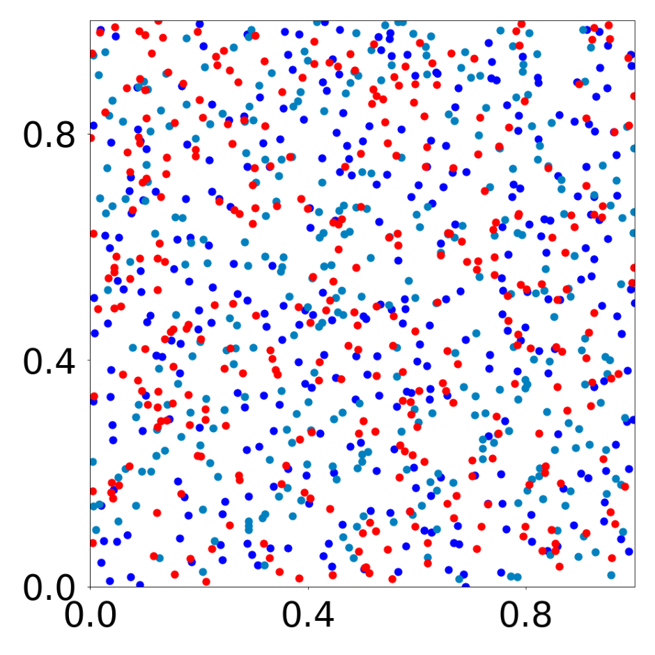
This script creates the third column of paper’s Figure 2. Simulation of a Coulomb-like system: 960 particles, 3 different charges.
First, we load the configuration file and set the device.
The following model is used to simulate the Coulomb-like system with PyTorch Geometric. There are three possible charges: -1, 1, and 2.
class CoulombModel(pyg.nn.MessagePassing):
        """Interaction Network as proposed in this paper:
        https://proceedings.neurips.cc/paper/2016/hash/3147da8ab4a0437c15ef51a5cc7f2dc4-Abstract.html"""

        """
        Compute the acceleration of charged particles as a function of their relative position according to the Coulomb law.

        Inputs
        ----------
        data : a torch_geometric.data object

        Returns
        -------
        pred : float
            the acceleration of the particles (dimension 2)
        """

        def __init__(self, aggr_type=[], p=[], clamp=[], pred_limit=[], bc_dpos=[]):
            super(CoulombModel, self).__init__(aggr='add')  # "mean" aggregation.

            self.p = p
            self.clamp = clamp
            self.pred_limit = pred_limit
            self.bc_dpos = bc_dpos

        def forward(self, data):
            x, edge_index = data.x, data.edge_index
            edge_index, _ = pyg_utils.remove_self_loops(edge_index)
            particle_type = to_numpy(x[:, 5])
            charge = self.p[particle_type]
            dd_pos = self.propagate(edge_index, pos=x[:, 1:3], charge=charge[:, None])
            return dd_pos

        def message(self, pos_i, pos_j, charge_i, charge_j):
            distance_ij = torch.sqrt(torch.sum(self.bc_dpos(pos_j - pos_i) ** 2, axis=1))
            direction_ij = self.bc_dpos(pos_j - pos_i) / distance_ij[:, None]
            dd_pos = - charge_i * charge_j * direction_ij / (distance_ij[:, None] ** 2)
            return dd_pos


def bc_pos(x):
    return torch.remainder(x, 1.0)


def bc_dpos(x):
    return torch.remainder(x - 0.5, 1.0) - 0.5
The data is generated with the above Pytorch Geometric model. Note two datasets are generated, one for training and one for validation. If the simulation is too large, you can decrease n_particles (multiple of 3) in “Coulomb_3_256.yaml”.#
p = torch.squeeze(torch.tensor(config.simulation.params))
model = CoulombModel(aggr_type=config.graph_model.aggr_type, p=torch.squeeze(p),
                          clamp=config.training.clamp, pred_limit=config.training.pred_limit, bc_dpos=bc_dpos)

generate_kwargs = dict(device=device, visualize=True, run_vizualized=0, style='color', alpha=1, erase=True, save=True, step=10)
train_kwargs = dict(device=device, erase=True)
test_kwargs = dict(device=device, visualize=True, style='color', verbose=False, best_model='20', run=0, step=1, save_velocity=True)

data_generate_particles(config, model, bc_pos, bc_dpos, **generate_kwargs)
Finally, we generate the figures that are shown in Figure 2. All frames are saved in ‘decomp-gnn/paper_experiments/graphs_data/graphs_Coulomb_3_256/Fig/’.