Attraction-repulsion system with 3 particle types

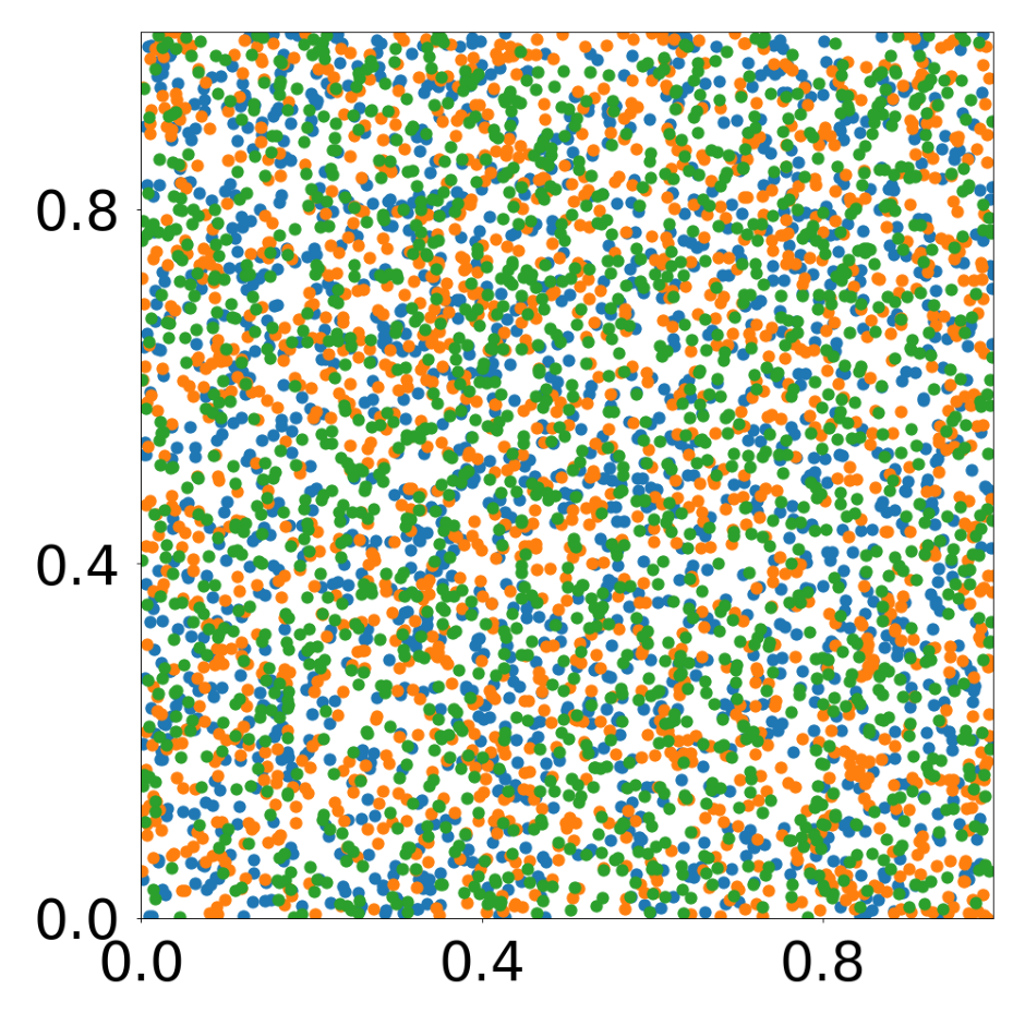
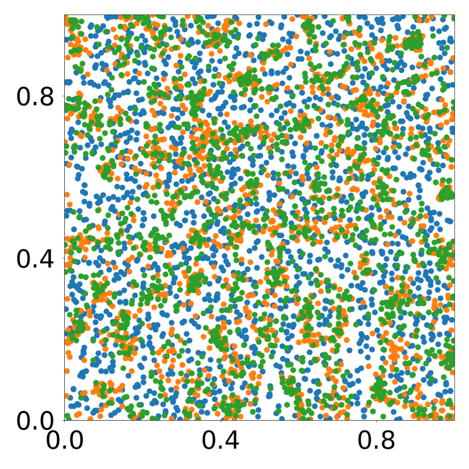
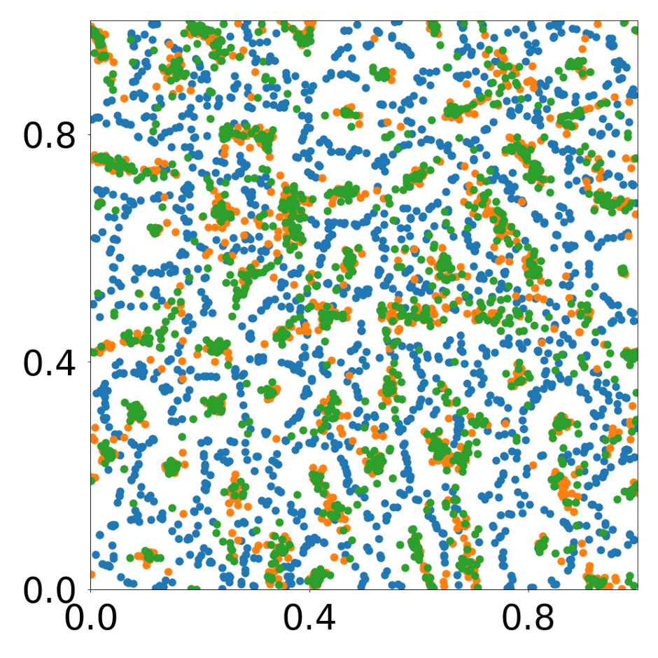
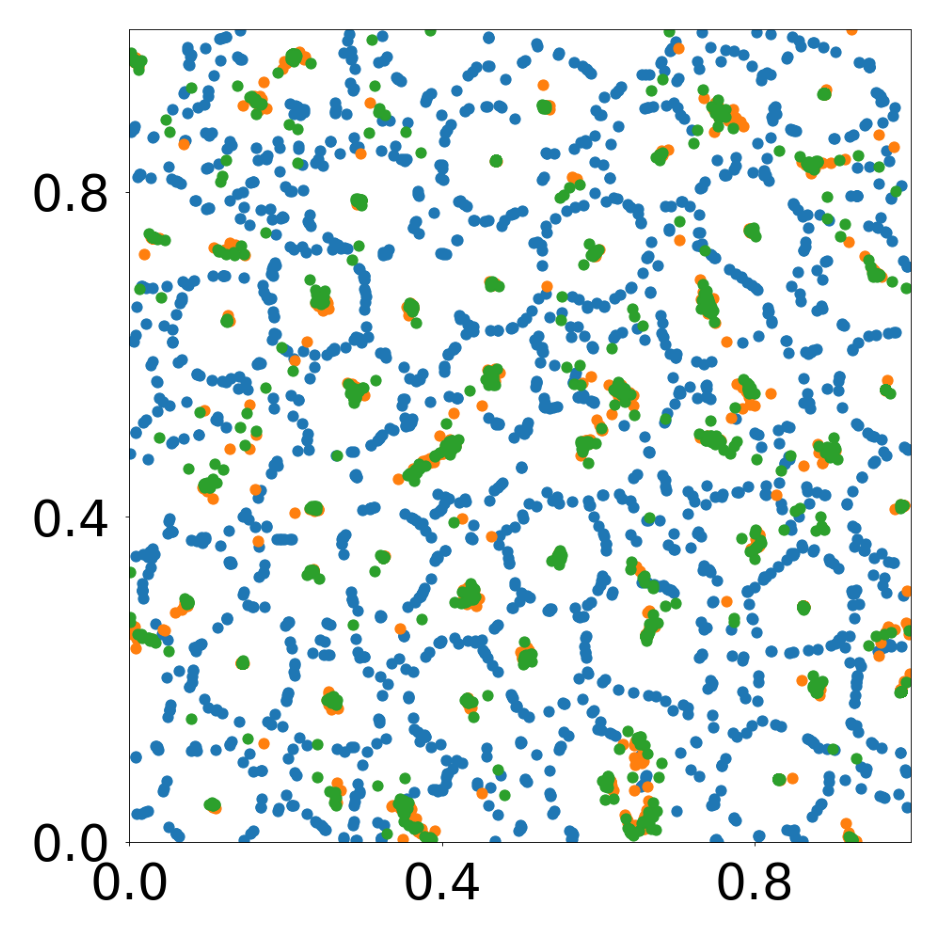
This script creates the first column of paper’s Figure 2. Simulation of an attraction-repulsion system, 4800 particles, 3 particle types.

First, we load the configuration file and set the device.

config_file = 'arbitrary_3'
config = ParticleGraphConfig.from_yaml(f'./config/{config_file}.yaml')
device = set_device("auto")

The following model is used to simulate the attraction-repulsion system with PyTorch Geometric.

class AttractionRepulsionModel(pyg.nn.MessagePassing):
    """
    Compute the speed of particles as a function of their relative position according to an attraction-repulsion law.
    The latter is defined by four parameters p = (p1, p2, p3, p4) and a parameter sigma.

    See https://github.com/gpeyre/numerical-tours/blob/master/python/ml_10_particle_system.ipynb
    """

    def __init__(self, p, sigma, bc_dpos, dimension=2):
        super(AttractionRepulsionModel, self).__init__(aggr='mean')

        self.p = p
        self.sigma = sigma
        self.bc_dpos = bc_dpos
        self.dimension = dimension

    def forward(self, data: Data):
        x, edge_index = data.x, data.edge_index

        edge_index, _ = pyg_utils.remove_self_loops(edge_index)
        particle_type = to_numpy(x[:, 1 + 2 * self.dimension])
        parameters = self.p[particle_type,:]
        d_pos = self.propagate(edge_index, pos=x[:, 1:self.dimension + 1], parameters=parameters)
        return d_pos

    def message(self, pos_i, pos_j, parameters_i):

        relative_position = self.bc_dpos(pos_j - pos_i)
        distance_squared = torch.sum(relative_position ** 2, dim=1)  # squared distance
        f = (parameters_i[:, 0] * torch.exp(-distance_squared ** parameters_i[:, 1] / (2 * self.sigma ** 2))
             - parameters_i[:, 2] * torch.exp(-distance_squared ** parameters_i[:, 3] / (2 * self.sigma ** 2)))
        velocity = f[:, None] * relative_position

        return velocity


def bc_pos(x):
    return torch.remainder(x, 1.0)


def bc_dpos(x):
    return torch.remainder(x - 0.5, 1.0) - 0.5

The data is generated with the above Pytorch Geometric model. Note two datasets are generated, one for training and one for validation. If the simulation is too large, you can decrease n_particles (multiple of 3) in “arbitrary_3.yaml”.

p = torch.squeeze(torch.tensor(config.simulation.params))
sigma = config.simulation.sigma
model = AttractionRepulsionModel(
    p=p,
    sigma=sigma,
    bc_dpos=bc_dpos,
    dimension=config.simulation.dimension
)

generate_kwargs = dict(device=device, visualize=True, run_vizualized=0, style='color', alpha=1, erase=True, save=True, step=10)
train_kwargs = dict(device=device, erase=True)
test_kwargs = dict(device=device, visualize=True, style='color', verbose=False, best_model='20', run=0, step=1, save_velocity=True)

data_generate_particles(config, model, bc_pos, bc_dpos, **generate_kwargs)

Finally, we generate the figures that are shown in Figure 2. All frames are saved in ‘decomp-gnn/paper_experiments/graphs_data/arbitrary_3/Fig/’.

Initial configuration of the simulation. There are 4800 particles. The orange, blue, and green particles represent the three different particle types.

Frame 80 out 250

Frame 160 out 250

Frame 240 out 250