Figure 3: External Inputs - 2048 neurons with external inputs

This script reproduces paper’s Figure 3. We tested whether we could recover both network structure and dynamics, as well as unknown external inputs

Simulation parameters:

• N_neurons: 2048 (1024 with external inputs + 1024 without)
• N_types: 4 (parameterized by \(\tau_i\)={0.5,1}, \(s_i\)={1,2}, \(\gamma_j\)={1,2,4,8})
• N_frames: 50,000
• Connectivity: 100% (dense)
• Noise \(\eta_i(t)\): Gaussian, variance \(\sigma^2=7.2\)
• External inputs: \(\Omega_i(t)\) - time-dependent scalar field \(\Omega_i(t)\)

The simulation follows:

\[\frac{dx_i}{dt} = -\frac{x_i}{\tau_i} + s_i \tanh(x_i) + g_i \Omega_i(t) \sum_j W_{ij} \tanh\left(\frac{x_j}{\gamma_j}\right) + \eta_i(t)\]

The GNN learns:

\[\hat{\dot{x}}_i = \phi^*(\mathbf{a}_i, x_i) + \Omega_i^*(t) \sum_j W_{ij} \psi^*(\mathbf{a}_j, x_j)\]

The external input \(\Omega_i(t)\) is scalar field that modulates the connectivity for the first 1024 neurons. The neuron index \(i\) corresponds to a known spatial coordinate \(x_i\). The remaining 1024 neurons have \(\Omega_i = 1\).

Configuration and Setup

print()
print("=" * 80)
print("Figure 3: 2048 neurons, 4 types, with external inputs Omega(t)")
print("=" * 80)

device = []
best_model = ''
config_file_ = 'signal_fig_3'

print()
config_root = "./config"
config_file, pre_folder = add_pre_folder(config_file_)

# load config
config = NeuralGraphConfig.from_yaml(f"{config_root}/{config_file}.yaml")
config.config_file = config_file
config.dataset = config_file

if device == []:
    device = set_device(config.training.device)

log_dir = f'./log/{config_file}'
graphs_dir = f'./graphs_data/{config_file}'

Step 1: Generate Data

Generate synthetic neural activity data using the PDE_N4 model. This creates the training dataset with 2048 neurons and external inputs.

Outputs:

• Figure 3a: External inputs Omega_i(t) - time-dependent scalar field
• Figure 3b: Activity time series
• Figure 3c: Sample of 100 time series

# STEP 1: GENERATE
print()
print("-" * 80)
print("STEP 1: GENERATE - Simulating neural activity with external inputs (Fig 3a-c)")
print("-" * 80)

# Check if data already exists
data_file = f'{graphs_dir}/x_list_0.npy'
if os.path.exists(data_file):
    print(f"data already exists at {graphs_dir}/")
    print("skipping simulation, regenerating figures...")
    data_generate(
        config,
        device=device,
        visualize=False,
        run_vizualized=0,
        style="color",
        alpha=1,
        erase=False,
        bSave=True,
        step=2,
        regenerate_plots_only=True,
    )
else:
    print(f"simulating {config.simulation.n_neurons} neurons, {config.simulation.n_neuron_types} types")
    print(f"external inputs: {config.simulation.n_input_neurons} neurons modulated by Omega(t)")
    print(f"generating {config.simulation.n_frames} time frames")
    print(f"output: {graphs_dir}/")
    print()
    data_generate(
        config,
        device=device,
        visualize=False,
        run_vizualized=0,
        style="color",
        alpha=1,
        erase=False,
        bSave=True,
        step=2,
    )

Fig 3a-b: (Top) External input field \(\Omega_i(t)\) shown on a 32×32 grid (left, first 1024 neurons) and sunflower arrangement (right, remaining 1024 neurons). (Bottom) Neural activity \(x_i\) at time \(t=0\).

Fig 3c: Sample activity time series for 100 neurons over 10,000 time steps. Y-axis shows neuron index.

Step 2: Train GNN

Train the GNN to learn connectivity \(W\), latent embeddings \(\mathbf{a}_i\), functions \(\phi^*/\psi^*\), and the external input field \(\Omega^*(x, y, t)\) using a coordinate-based MLP (SIREN).

Learning targets:

• Connectivity matrix \(W\)
• Latent vectors \(\mathbf{a}_i\)
• Update function \(\phi^*(\mathbf{a}_i, x)\)
• Transfer function \(\psi^*(x)\)
• External input field \(\Omega^*(x, y, t)\) via SIREN network

# STEP 2: TRAIN
print()
print("-" * 80)
print("STEP 2: TRAIN - Training GNN to learn W, embeddings, phi, psi, and Omega*")
print("-" * 80)

# Check if trained model already exists (any .pt file in models folder)
import glob
model_files = glob.glob(f'{log_dir}/models/*.pt')
if model_files:
    print(f"trained model already exists at {log_dir}/models/")
    print("skipping training (delete models folder to retrain)")
else:
    print(f"training for {config.training.n_epochs} epochs, {config.training.n_runs} run(s)")
    print(f"learning: connectivity W, latent vectors a_i, functions phi*, psi*")
    print(f"learning: external input field Omega*(x, y, t) via SIREN network")
    print(f"models: {log_dir}/models/")
    print(f"training plots: {log_dir}/tmp_training")
    print(f"tensorboard: tensorboard --logdir {log_dir}/")
    print()
    data_train(
        config=config,
        erase=False,
        best_model=best_model,
        style='color',
        device=device
    )

Step 3: Generate Publication Figures

Generate publication-quality figures matching Figure 3 from the paper.

Figure panels:

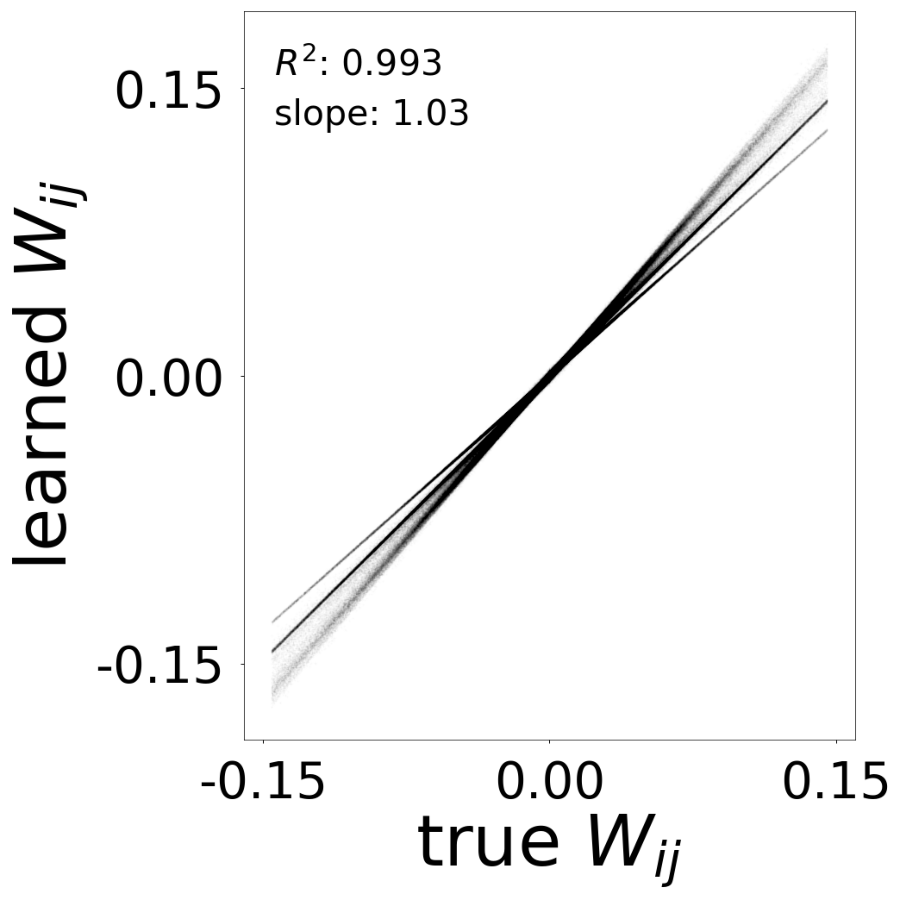
• Fig 3d: Comparison of learned vs true connectivity W_ij
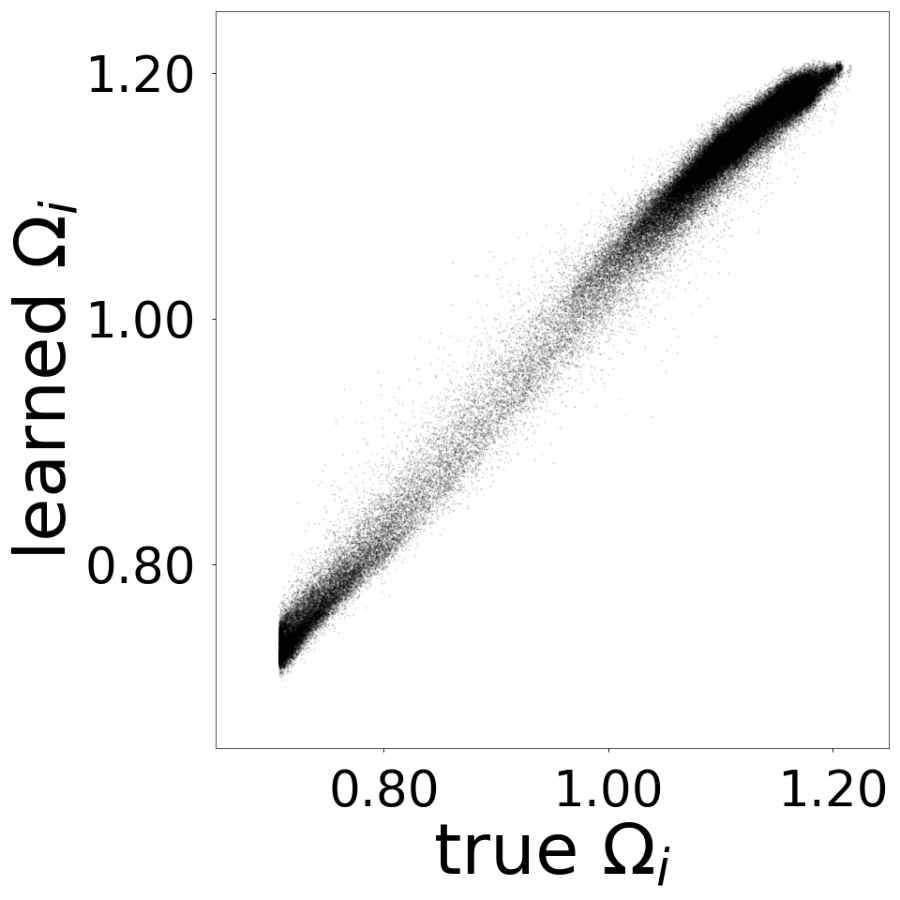
• Fig 3e: Comparison of learned vs true Omega_i(t) values
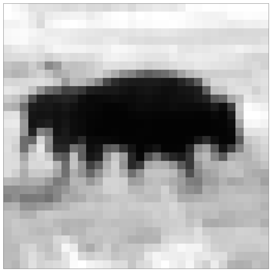
• Fig 3f: True field Omega_i(t) at different time-points
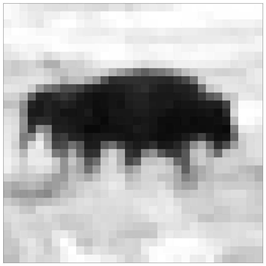
• Fig 3g: Learned field Omega*(t) at different time-points

# STEP 3: PLOT
print()
print("-" * 80)
print("STEP 3: PLOT - Generating Figure 3 panels (d-g)")
print("-" * 80)
print(f"Fig 3d: W learned vs true (R^2, slope)")
print(f"Fig 3e: Omega learned vs true")
print(f"Fig 3f: True field Omega_i(t) at different times")
print(f"Fig 3g: Learned field Omega*(t) at different times")
print(f"output: {log_dir}/results/")
print()
folder_name = './log/' + pre_folder + '/tmp_results/'
os.makedirs(folder_name, exist_ok=True)
data_plot(config=config, config_file=config_file, epoch_list=['best'], style='color', extended='plots', device=device, apply_weight_correction=True, plot_eigen_analysis=False)

Output Files

Rename output files to match Figure 3 panels.

# Rename output files to match Figure 3 panels
print()
print("-" * 80)
print("renaming output files to Figure 3 panels")
print("-" * 80)

results_dir = f'{log_dir}/results'
os.makedirs(results_dir, exist_ok=True)

# File mapping for simple copies
file_mapping = {
    f'{graphs_dir}/activity_sample.png': f'{results_dir}/Fig3d_activity_sample.png',
    f'{results_dir}/weights_comparison_corrected.png': f'{results_dir}/Fig3e_weights_comparison.png',
}

for src, dst in file_mapping.items():
    if os.path.exists(src):
        shutil.copy2(src, dst)
        print(f"{os.path.basename(dst)}")

import glob
import numpy as np
import matplotlib.pyplot as plt
import matplotlib.image as mpimg

# Copy Fig 3a-b from generated frame (plot_synaptic_frame_visual output)
fig_file = f'{graphs_dir}/Fig/Fig_0_000000.png'
if os.path.exists(fig_file):
    shutil.copy2(fig_file, f'{results_dir}/Fig3ab_external_input_activity.png')
    print(f"Fig3ab_external_input_activity.png")

# Copy Fig 3c: Activity time series
if os.path.exists(f'{graphs_dir}/activity.png'):
    shutil.copy2(f'{graphs_dir}/activity.png', f'{results_dir}/Fig3c_activity_time_series.png')
    print(f"Fig3c_activity_time_series.png")

# Generate Fig 3f: True field Omega_i(t) montage from field images
print("generating Fig3f_omega_field_true.png (5-frame montage)...")
field_dir = f'{results_dir}/field'
frame_indices = [0, 10000, 20000, 30000, 40000]

fig, axes = plt.subplots(1, 5, figsize=(20, 4))
for idx, frame in enumerate(frame_indices):
    ax = axes[idx]
    # Find true field image for this frame
    true_field_files = sorted(glob.glob(f'{field_dir}/true_field*_{frame}.png'))
    if true_field_files:
        img = mpimg.imread(true_field_files[-1])
        ax.imshow(img, cmap='gray')
    ax.set_xticks([])
    ax.set_yticks([])
    ax.set_title(f't={frame}', fontsize=12)
    ax.axis('off')
plt.tight_layout()
plt.savefig(f'{results_dir}/Fig3f_omega_field_true.png', dpi=150)
plt.close()
print(f"Fig3f_omega_field_true.png")

# Generate Fig 3g: Learned field Omega*(t) montage from field images
print("generating Fig3g_omega_field_learned.png (5-frame montage)...")
fig, axes = plt.subplots(1, 5, figsize=(20, 4))
for idx, frame in enumerate(frame_indices):
    ax = axes[idx]
    # Find learned field image for this frame
    learned_field_files = sorted(glob.glob(f'{field_dir}/reconstructed_field_LR*_{frame}.png'))
    if learned_field_files:
        img = mpimg.imread(learned_field_files[-1])
        ax.imshow(img, cmap='gray')
    ax.set_xticks([])
    ax.set_yticks([])
    ax.set_title(f't={frame}', fontsize=12)
    ax.axis('off')
plt.tight_layout()
plt.savefig(f'{results_dir}/Fig3g_omega_field_learned.png', dpi=150)
plt.close()
print(f"Fig3g_omega_field_learned.png")

print()
print("=" * 80)
print("Figure 3 complete!")
print(f"results saved to: {log_dir}/results/")
print("=" * 80)

Figure 3 Panels

Fig 3d: Comparison of learned and true connectivity.

Fig 3e: Comparison of learned and true \(\Omega_i\) values.

Fig 3f-g: True and Learned External Input Fields

Showing \(\Omega_i(t)\) at frames 0, 10000, 20000, 30000, 40000.

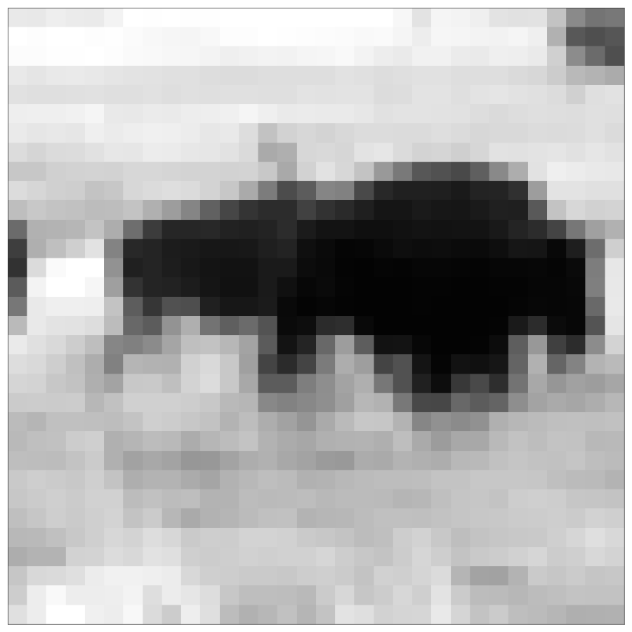
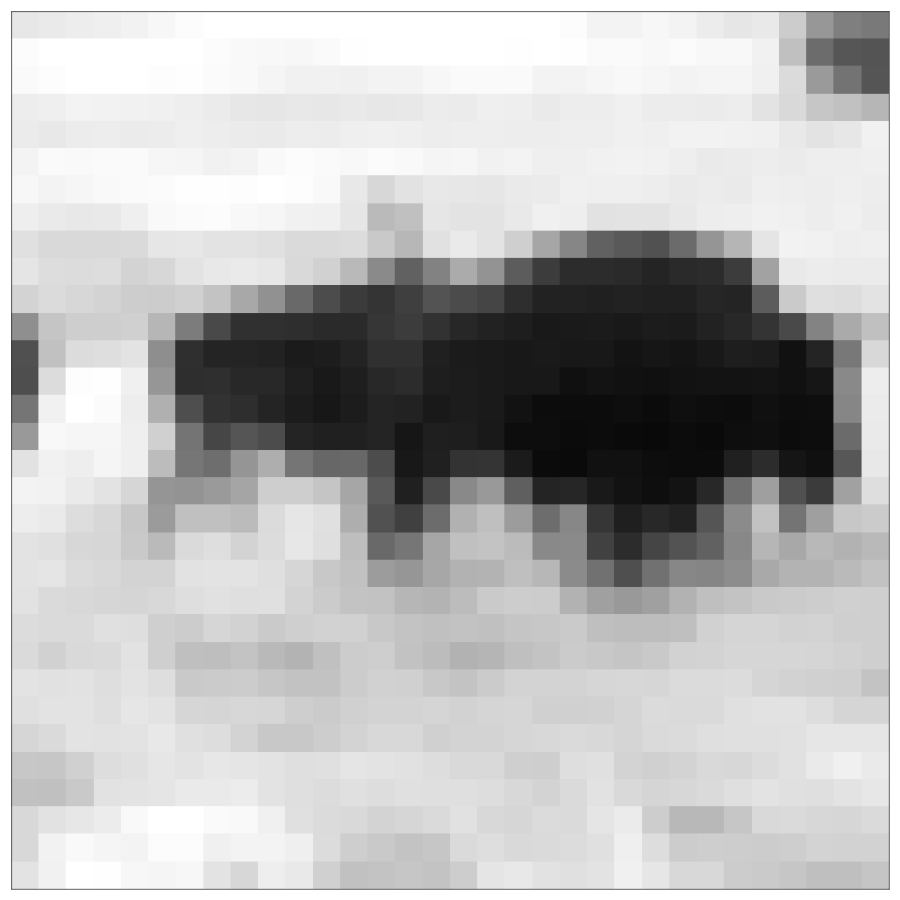
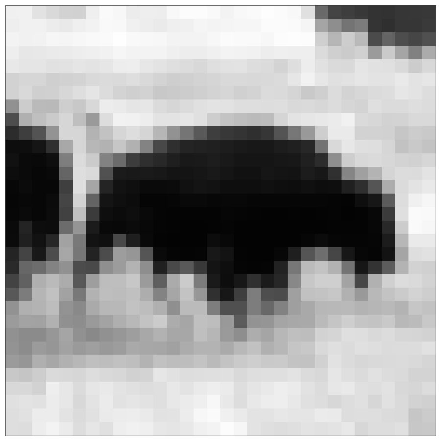
True field \(\Omega_i\) at frame 0.

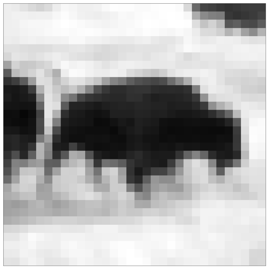
Learned field \(\Omega^*_i\) at frame 0.

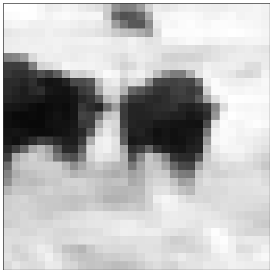
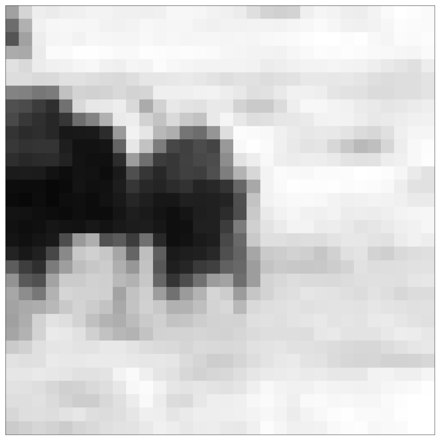
True field \(\Omega_i\) at frame 10000.

Learned field \(\Omega^*_i\) at frame 10000.

True field \(\Omega_i\) at frame 20000.

Learned field \(\Omega^*_i\) at frame 20000.

True field \(\Omega_i\) at frame 30000.

Learned field \(\Omega^*_i\) at frame 30000.

True field \(\Omega_i\) at frame 40000.

Learned field \(\Omega^*_i\) at frame 40000.

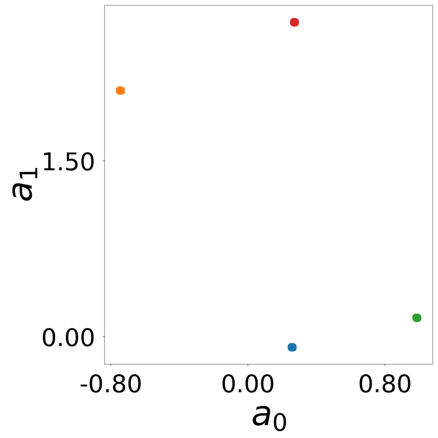
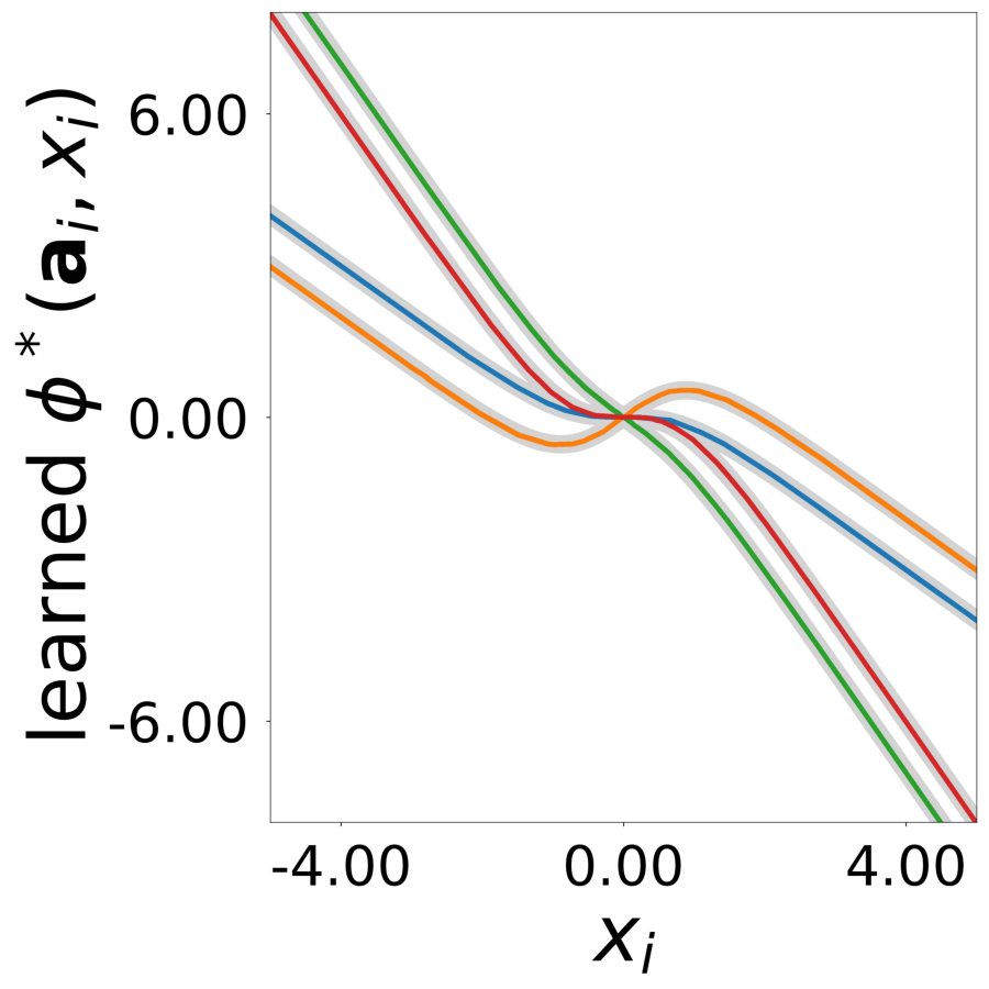
Supplementary Figure 15: Learned Functions

Learned latent embeddings and functions from Figure 3 training.

Supp. Fig 15f: Learned latent vectors \(a_i\).

Supp. Fig 15g: Learned update functions \(\phi^*(a, x)\). Colors indicate true neuron types. True functions are overlaid in light gray.

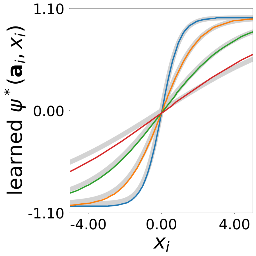
Supp. Fig 15h: : Learned transfer function \(\psi^*(x)\), normalized to a maximum value of 1. True functions are overlaid in light gray.