This script reproduces the panels of paper’s Supplementary Figure 14. Training with neuron-neuron dependent transfer functions of the form \(\psi(a_i, a_j, x_j)\).
Simulation parameters:
N_neurons: 1000
N_types: 4 parameterized by \(\tau_i\)={0.5,1}, \(s_i\)={1,2} and \(g_i\)=10
N_frames: 100,000
Connectivity: 100% (dense)
Connectivity weights: random, Lorentz distribution
Noise: none
External inputs: none
Transfer function \(\gamma_i\)={1,2,4,8} (receiver-dependent)
Linear slope \(\theta_j\)={0, 0.013, 0.027, 0.040} (sender-dependent)
The simulation follows an extended version of Equation 2:
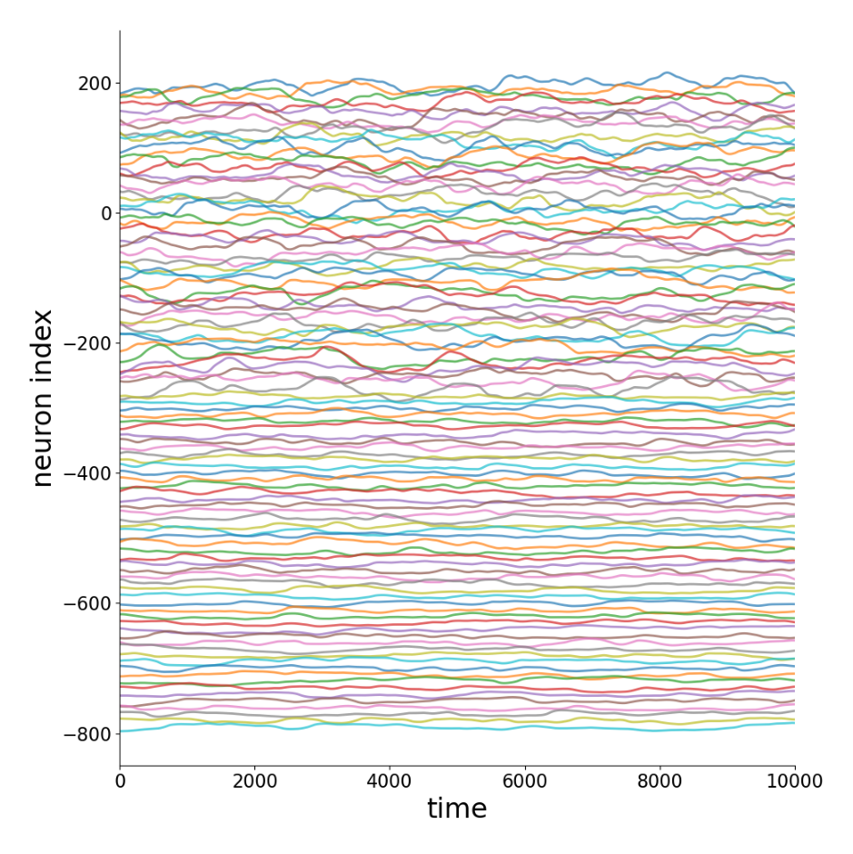
Generate synthetic neural activity data using the PDE_N5 model with neuron-dependent transfer functions. Each pair of neuron types has different transfer function characteristics depending on both source (\(a_j\)) and target (\(a_i\)) embeddings.
Train the GNN to learn connectivity \(W\), latent embeddings \(\mathbf{a}_i\), and functions \(\phi^*, \psi^*\). The GNN must learn neuron-neuron dependent transfer functions \(\psi^*(\mathbf{a}_i, \mathbf{a}_j, x_j)\).
Code
# STEP 2: TRAINprint()print("-"*80)print("STEP 2: TRAIN - Training GNN to learn neuron-dependent transfer functions")print("-"*80)# Check if trained model already exists (any .pt file in models folder)import globmodel_files = glob.glob(f'{log_dir}/models/*.pt')if model_files:print(f"trained model already exists at {log_dir}/models/")print("skipping training (delete models folder to retrain)")else:print(f"training for {config.training.n_epochs} epochs, {config.training.n_runs} run(s)")print(f"learning: connectivity W, latent vectors a_i, neuron-dependent psi*(a_i, a_j, x_j)")print(f"models: {log_dir}/models/")print(f"training plots: {log_dir}/tmp_training")print(f"tensorboard: tensorboard --logdir {log_dir}/")print() data_train( config=config, erase=False, best_model=best_model, style='color', device=device )
Step 3: GNN Evaluation
Figures matching Supplementary Figure 14 from the paper.
Figure panels:
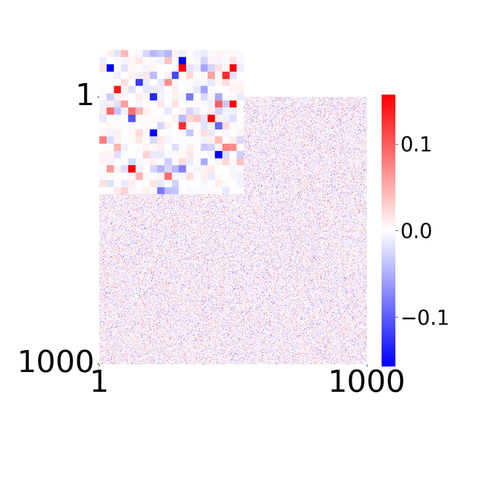
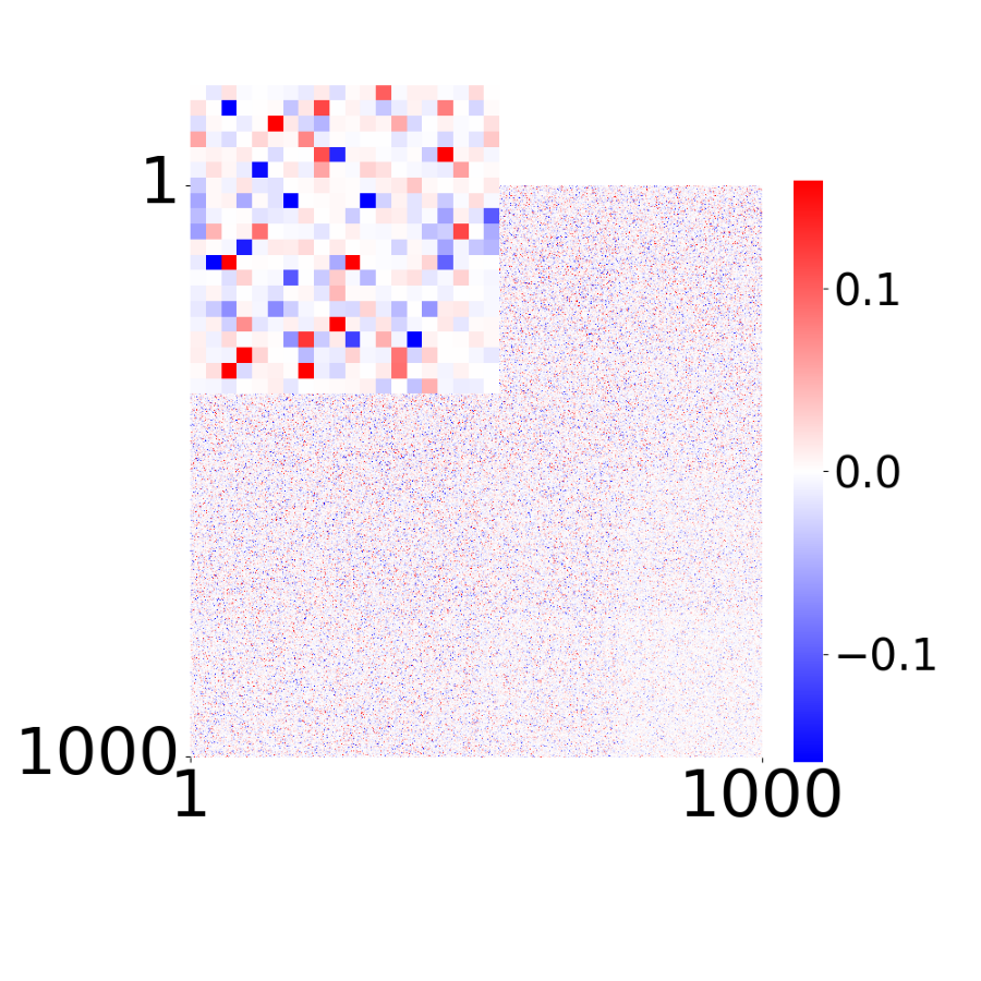
Supp. Fig 14d: Learned connectivity
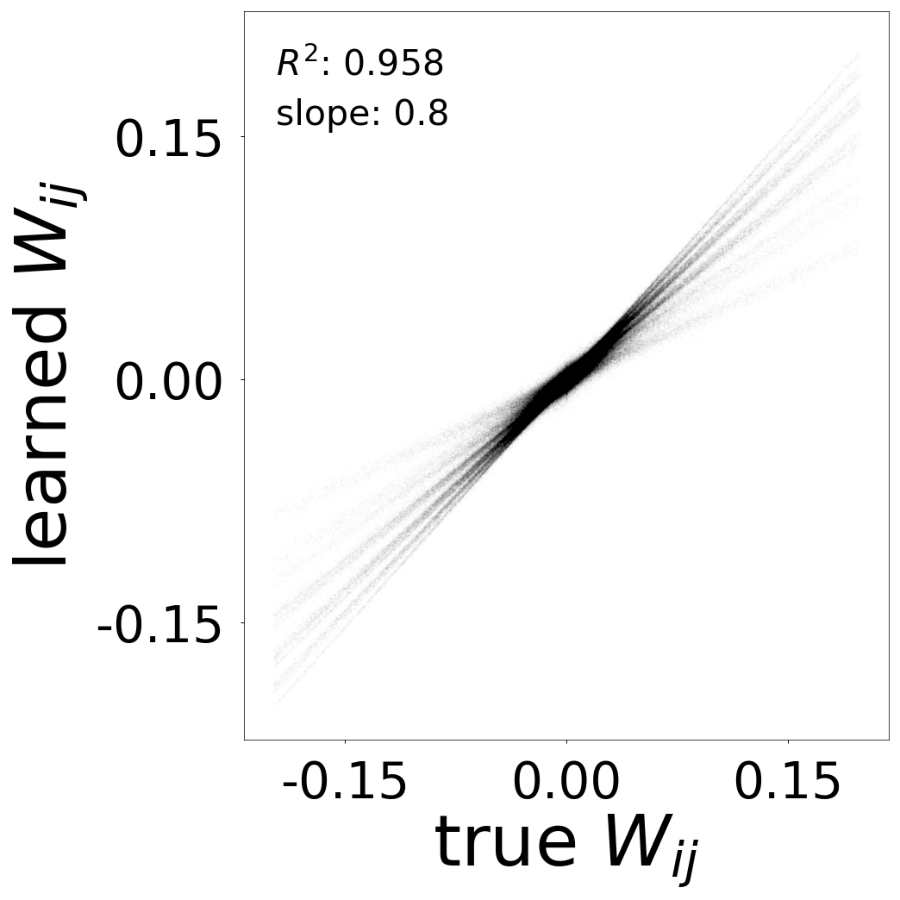
Supp. Fig 14e: Comparison between learned and true connectivity
Supp. Fig 14e: Comparison of learned and true connectivity (given \(g_i\)=10). Expected: \(R^2\)=0.99, slope=0.99.
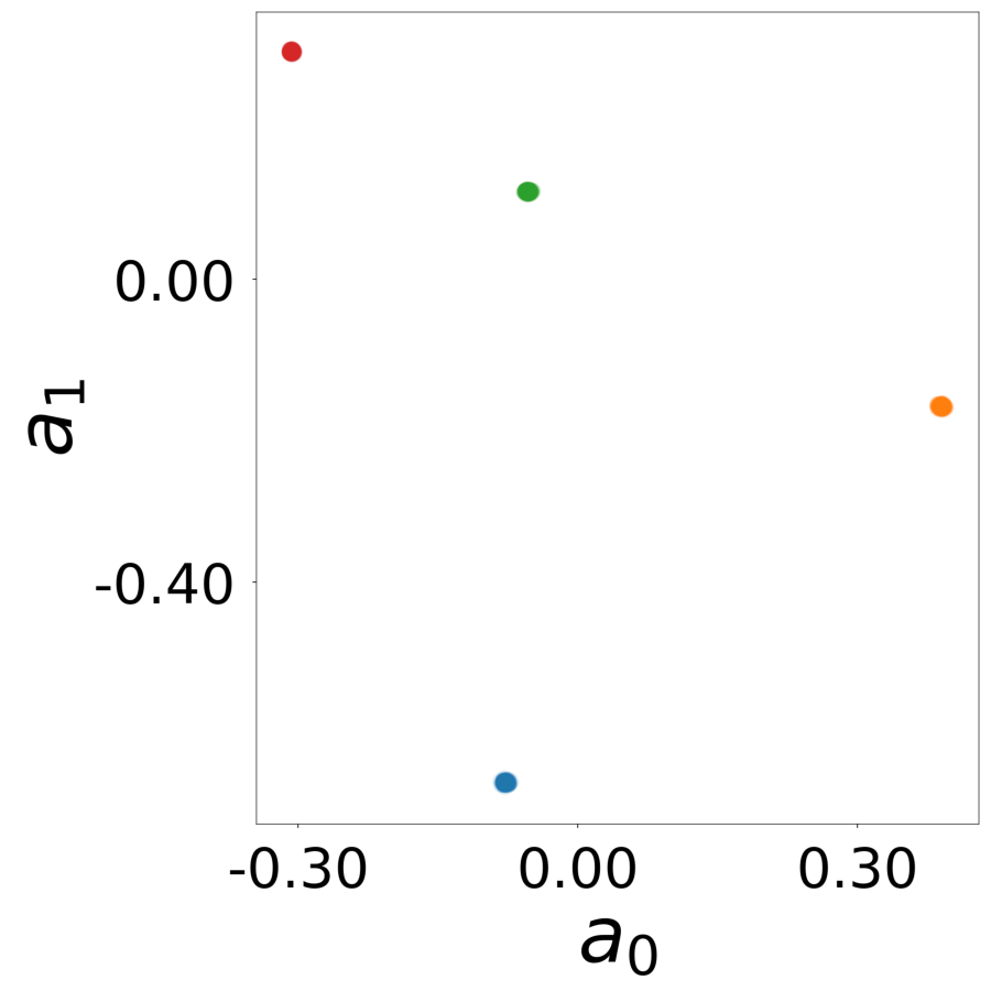
Supp. Fig 14f: Learned latent vectors \(a_i\) of all neurons.
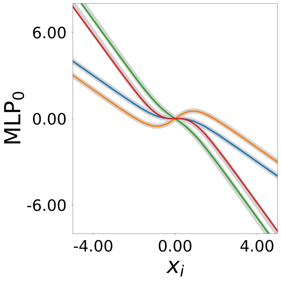
Supp. Fig 14g: Learned update functions \(\phi^*(a_i, x)\). The plot shows 1000 overlaid curves. Colors indicate true neuron types. True functions are overlaid in light gray.
Supp. Fig 14h: Learned transfer functions \(\psi^*(a_i, a_j, x_j)\). 2x2 montage: each panel corresponds to a receiving neuron type (border color), showing curves for all sending neuron types (line colors). True functions in gray.