This script reproduces the panels of paper’s Supplementary Figure 13 . Test with neuron-specific transfer functions of the form \(\psi(x_j/\gamma_i)\) .
Simulation parameters:
N_neurons: 1000
N_types: 4 parameterized by \(\tau_i\) ={0.5,1}, \(s_i\) ={1,2} and \(g_i\) =10
N_frames: 100,000
Connectivity: 100% (dense)
Connectivity weights: random, Lorentz distribution
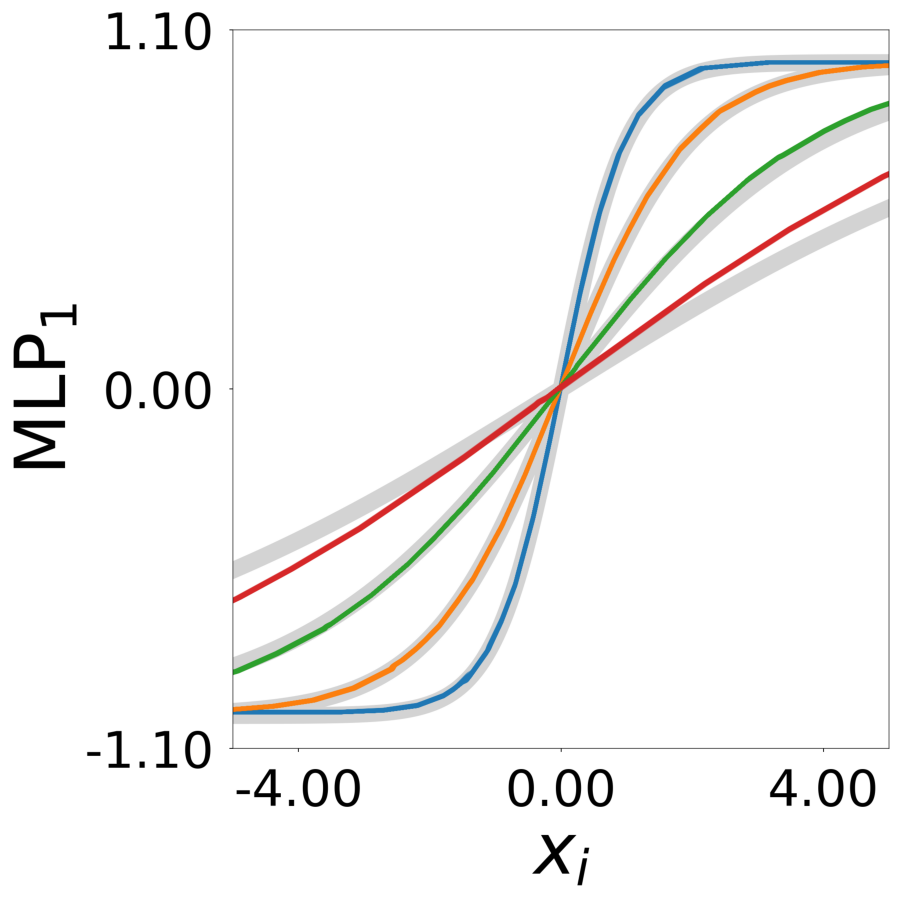
Transfer function \(\gamma_i\) ={1,2,4,8} (neuron-specific)
The simulation follows an extended version of Equation 2:
\[\frac{dx_i}{dt} = -\frac{x_i}{\tau_i} + s_i \cdot \tanh(x_i) + g_i \cdot \sum_j W_{ij} \cdot \tanh\left(\frac{x_j}{\gamma_i}\right)\]
The GNN jointly optimizes the shared MLP \(\psi^*\) and latent vectors \(\mathbf{a}_i\) to accurately identify the neuron-specific transfer functions.
Configuration and Setup
Code
print ()print ("=" * 80 )print ("Supplementary Figure 13: 1000 neurons, 4 types, heterogeneous transfer functions" )print ("=" * 80 )= []= '' = 'signal_fig_supp_13' print ()= "./config" = add_pre_folder(config_file_)# load config = NeuralGraphConfig.from_yaml(f" { config_root} / { config_file} .yaml" )= config_file= config_fileif device == []:= set_device(config.training.device)= f'./log/ { config_file} ' = f'./graphs_data/ { config_file} '
Step 1: Generate Data
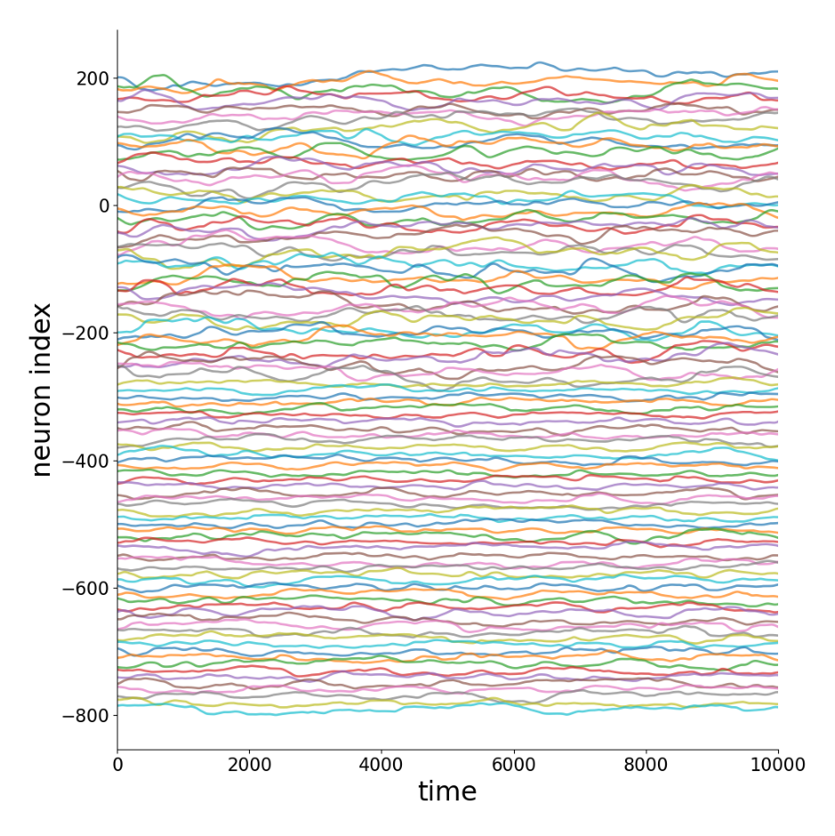
Generate synthetic neural activity data using the PDE_N4 model with neuron-specific transfer functions. Each neuron type has a different parameter \(\gamma_i\) in the transfer function \(\psi(x_j/\gamma_i)\) .
Outputs:
Sample time series
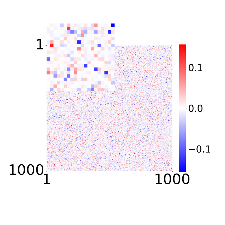
True connectivity matrix \(W_{ij}\)
Code
# STEP 1: GENERATE print ()print ("-" * 80 )print ("STEP 1: GENERATE - Simulating neural activity (heterogeneous transfer functions)" )print ("-" * 80 )# Check if data already exists = f' { graphs_dir} /x_list_0.npy' if os.path.exists(data_file):print (f"data already exists at { graphs_dir} /" )print ("skipping simulation, regenerating figures..." )= device,= False ,= 0 ,= "color" ,= 1 ,= False ,= True ,= 2 ,= True ,else :print (f"simulating { config. simulation. n_neurons} neurons, { config. simulation. n_neuron_types} types" )print (f"generating { config. simulation. n_frames} time frames" )print (f"transfer function gamma_i = [1, 2, 4, 8]" )print (f"output: { graphs_dir} /" )print ()= device,= False ,= 0 ,= "color" ,= 1 ,= False ,= True ,= 2 ,
Step 2: Train GNN
Train the GNN to learn connectivity \(W\) , latent embeddings \(\mathbf{a}_i\) , and functions \(\phi^*, \psi^*\) . The GNN must learn neuron-specific transfer functions \(\psi(x_j/\gamma_i)\) .
The GNN optimizes the update rule:
\[\hat{\dot{x}}_i = \phi^*(\mathbf{a}_i, x_i) + \sum_j W_{ij} \psi^*(\mathbf{a}_j, x_j)\]
where the transfer function \(\psi^*\) now depends on the latent vector \(\mathbf{a}_j\) .
Code
# STEP 2: TRAIN print ()print ("-" * 80 )print ("STEP 2: TRAIN - Training GNN to learn heterogeneous transfer functions" )print ("-" * 80 )# Check if trained model already exists (any .pt file in models folder) import glob= glob.glob(f' { log_dir} /models/*.pt' )if model_files:print (f"trained model already exists at { log_dir} /models/" )print ("skipping training (delete models folder to retrain)" )else :print (f"training for { config. training. n_epochs} epochs, { config. training. n_runs} run(s)" )print (f"learning: connectivity W, latent vectors a_i, neuron-specific psi*(a_j, x_j)" )print (f"models: { log_dir} /models/" )print (f"training plots: { log_dir} /tmp_training" )print (f"tensorboard: tensorboard --logdir { log_dir} /" )print ()= config,= False ,= best_model,= 'color' ,= device
Step 3: GNN Evaluation
Figures matching Supplementary Figure 13 from the paper.
Figure panels:
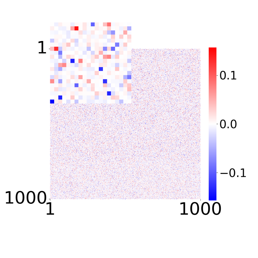
Supp. Fig 13d: Learned connectivity matrix
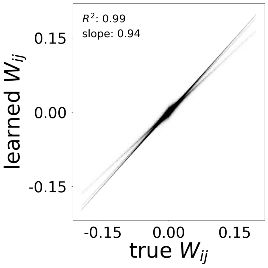
Supp. Fig 13e: Comparison of learned vs true connectivity (expected: \(R^2\) =0.99, slope=0.99)
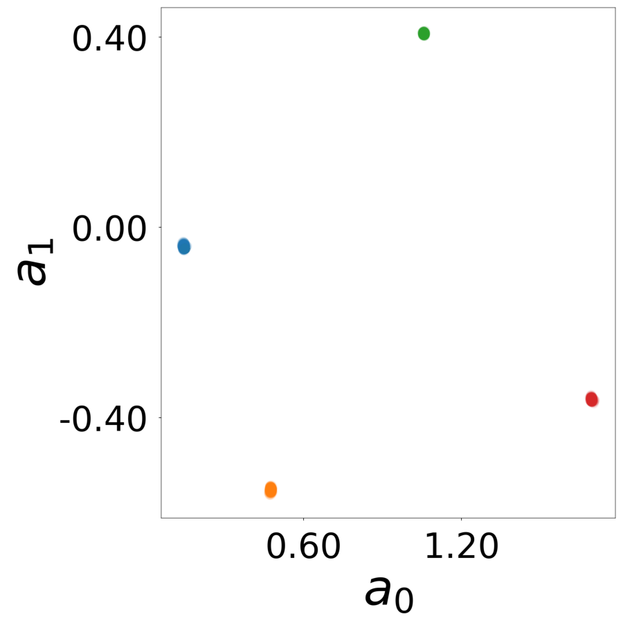
Supp. Fig 13f: Learned latent vectors \(\mathbf{a}_i\)
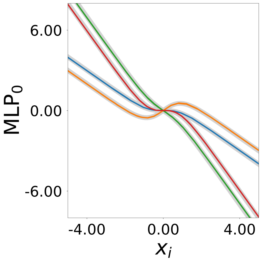
Supp. Fig 13g: Learned update functions \(\phi^*(\mathbf{a}_i, x)\)
Supp. Fig 13h: Learned transfer functions \(\psi^*(\mathbf{a}_j, x)\)
Code
# STEP 3: GNN EVALUATION print ()print ("-" * 80 )print ("STEP 3: GNN EVALUATION - Generating Supplementary Figure 13 panels" )print ("-" * 80 )print (f"learned connectivity matrix" )print (f"W learned vs true (R^2, slope)" )print (f"latent vectors a_i (4 clusters)" )print (f"update functions phi*(a_i, x)" )print (f"transfer functions psi*(a_j, x)" )print (f"output: { log_dir} /results/" )print ()= './log/' + pre_folder + '/tmp_results/' = True )= config, config_file= config_file, epoch_list= ['best' ], style= 'color' , extended= 'plots' , device= device, apply_weight_correction= True , plot_eigen_analysis= False )