Supplementary Figure 10: effect of Gaussian noise

This script reproduces the panels of paper’s Supplementary Figure 10. Gaussian noise is injected into the simulated dynamics (SNR of ∼10 dB).

Simulation parameters:

• N_neurons: 1000
• N_types: 4 parameterized by \(\tau_i\)={0.5,1}, \(s_i\)={1,2} and \(g_i\)=10
• N_frames: 100,000
• Connectivity: 100% (dense)
• Connectivity weights: random, Lorentz distribution
• Noise \(\eta_i(t)\): Gaussian, variance \(\sigma^2=7.2\)

The simulation follows Equation 2 from the paper:

\[\frac{dx_i}{dt} = -\frac{x_i}{\tau_i} + s_i \cdot \tanh(x_i) + g_i \cdot \sum_j W_{ij} \cdot \tanh(x_j) + \eta_i(t)\]

Configuration and Setup

print()
print("=" * 80)
print("Supplementary Figure 10: 1000 neurons, 4 types, dense connectivity, Gaussian noise")
print("=" * 80)

device = []
best_model = ''
config_file_ = 'signal_fig_supp_10'

print()
config_root = "./config"
config_file, pre_folder = add_pre_folder(config_file_)

# load config
config = NeuralGraphConfig.from_yaml(f"{config_root}/{config_file}.yaml")
config.config_file = config_file
config.dataset = config_file

if device == []:
    device = set_device(config.training.device)

log_dir = f'./log/{config_file}'
graphs_dir = f'./graphs_data/{config_file}'

Step 1: Generate Data

Generate synthetic neural activity data with Gaussian noise using the PDE_N2 model. This creates the training dataset with 1000 neurons of 4 different types over 100,000 time points.

Outputs:

• Supp. Fig 10b: Activity time series used for GNN training
• Supp. Fig 10c: True connectivity matrix \(W_{ij}\)

# STEP 1: GENERATE
print()
print("-" * 80)
print("STEP 1: GENERATE - Simulating neural activity with Gaussian noise")
print("-" * 80)

# Check if data already exists
data_file = f'{graphs_dir}/x_list_0.npy'
if os.path.exists(data_file):
    print(f"data already exists at {graphs_dir}/")
    print("skipping simulation, regenerating figures...")
    data_generate(
        config,
        device=device,
        visualize=False,
        run_vizualized=0,
        style="color",
        alpha=1,
        erase=False,
        bSave=True,
        step=2,
        regenerate_plots_only=True,
    )
else:
    print(f"simulating {config.simulation.n_neurons} neurons, {config.simulation.n_neuron_types} types")
    print(f"generating {config.simulation.n_frames} time frames with Gaussian noise")
    print(f"output: {graphs_dir}/")
    print()
    data_generate(
        config,
        device=device,
        visualize=False,
        run_vizualized=0,
        style="color",
        alpha=1,
        erase=False,
        bSave=True,
        step=2,
    )

Supp. Fig 10b: Sample of 100 time series taken from the activity data with Gaussian noise (~10 dB SNR).

Supp. Fig 10c: True connectivity \(W_{ij}\). The inset shows 20×20 weights.

Step 2: Train GNN

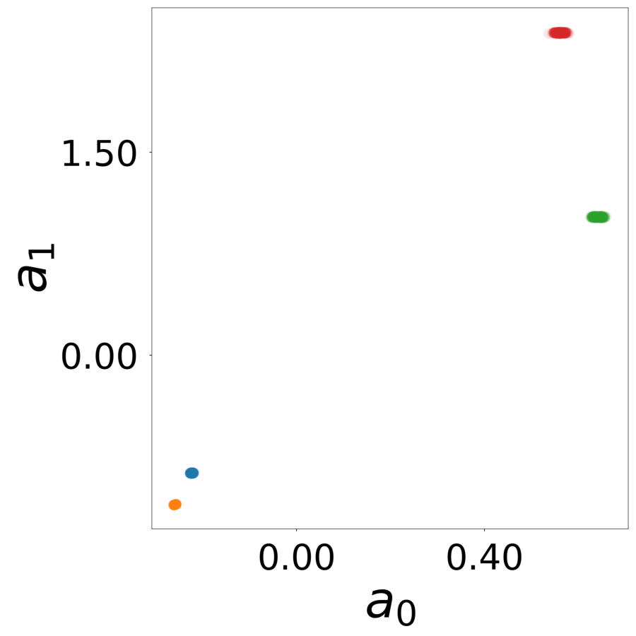
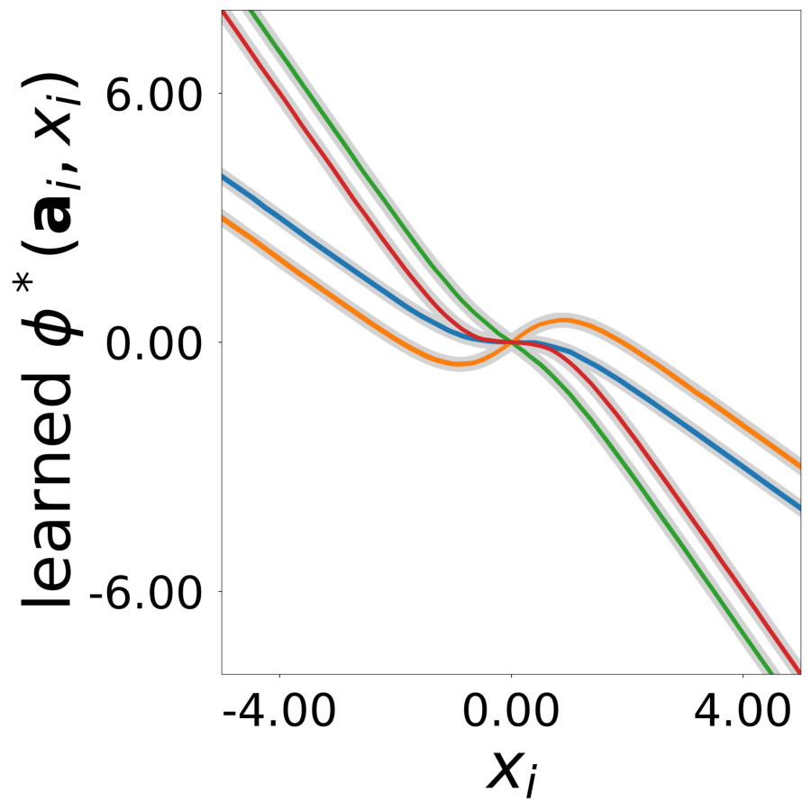
Train the GNN to learn connectivity \(W\), latent embeddings \(\mathbf{a}_i\), and functions \(\phi^*, \psi^*\). The GNN learns to predict \(dx_i/dt\) from the noisy observed activity \(x_i\).

The GNN optimizes the update rule (Equation 3 from the paper):

\[\hat{\dot{x}}_i = \phi^*(\mathbf{a}_i, x_i) + \sum_j W_{ij} \psi^*(x_j)\]

where \(\phi^*\) and \(\psi^*\) are MLPs (ReLU, hidden dim=64, 3 layers). \(\mathbf{a}_i\) is a learnable 2D latent vector per neuron, and \(W\) is the learnable connectivity matrix.

# STEP 2: TRAIN
print()
print("-" * 80)
print("STEP 2: TRAIN - Training GNN to learn W, embeddings, phi, psi from noisy data")
print("-" * 80)

# Check if trained model already exists (any .pt file in models folder)
import glob
model_files = glob.glob(f'{log_dir}/models/*.pt')
if model_files:
    print(f"trained model already exists at {log_dir}/models/")
    print("skipping training (delete models folder to retrain)")
else:
    print(f"training for {config.training.n_epochs} epochs, {config.training.n_runs} run(s)")
    print(f"learning: connectivity W, latent vectors a_i, functions phi* and psi*")
    print(f"models: {log_dir}/models/")
    print(f"training plots: {log_dir}/tmp_training")
    print(f"tensorboard: tensorboard --logdir {log_dir}/")
    print()
    data_train(
        config=config,
        erase=False,
        best_model=best_model,
        style='color',
        device=device
    )

Step 3: GNN Evaluation

Figures matching Supplementary Figure 10 from the paper.

Figure panels:

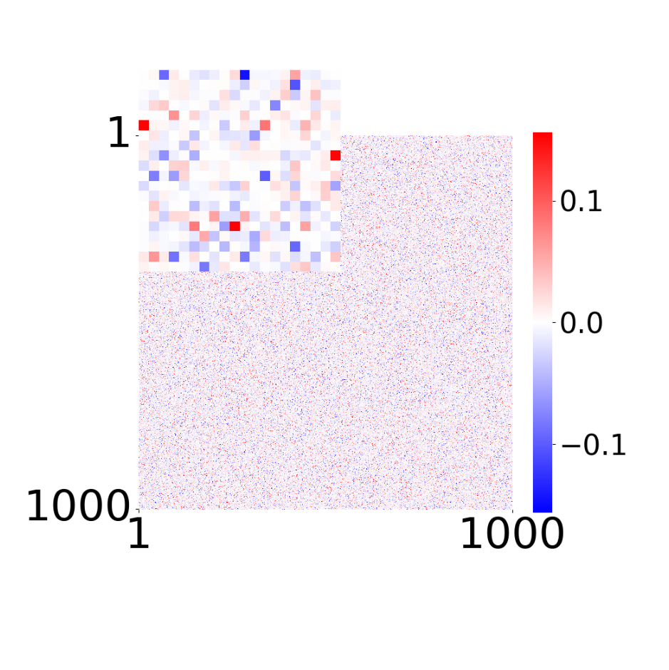
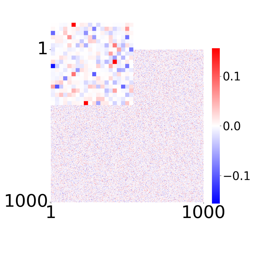
• Supp. Fig 10d: Learned connectivity matrix
• Supp. Fig 10e: Comparison of learned vs true connectivity
• Supp. Fig 10f: Learned latent vectors \(\mathbf{a}_i\)
• Supp. Fig 10g: Learned update functions \(\phi^*(\mathbf{a}_i, x)\)
• Supp. Fig 10h: Learned transfer function \(\psi^*(x)\)

# STEP 3: GNN EVALUATION
print()
print("-" * 80)
print("STEP 3: GNN EVALUATION - Generating Supplementary Figure 10 panels (d-h)")
print("-" * 80)
print(f"panel (d): Learned connectivity matrix")
print(f"panel (e): W learned vs true (R^2, slope)")
print(f"panel (f): Latent vectors a_i (4 clusters)")
print(f"panel (g): Update functions phi*(a_i, x)")
print(f"panel (h): Transfer function psi*(x)")
print(f"output: {log_dir}/results/")
print()
folder_name = './log/' + pre_folder + '/tmp_results/'
os.makedirs(folder_name, exist_ok=True)
data_plot(config=config, config_file=config_file, epoch_list=['best'], style='color', extended='plots', device=device, apply_weight_correction=True, plot_eigen_analysis=False)

Supplementary Figure 10: GNN Evaluation Results

Supp. Fig 10d: Learned connectivity.

Supp. Fig 10e: Comparison of learned and true connectivity (given \(g_i\)=10).

Supp. Fig 10f: Learned latent vectors \(a_i\) of all neurons.

Supp. Fig 10g: Learned update functions \(\phi^*(a_i, x)\). The plot shows 1000 overlaid curves, one for each vector \(a_i\). Colors indicate true neuron types. True functions are overlaid in light gray.

Supp. Fig 10h: Learned transfer function \(\psi^*(x)\), normalized to a maximum value of 1. True function is overlaid in light gray.