This script reproduces the panels of paper’s Supplementary Figures 3 and 4 . To assess the importance of learning latent neuron types, we trained a GNN with fixed embedding. Models that ignore the heterogeneity of neural populations are poor approximations of the underlying dynamics
Simulation parameters:
N_neurons: 1000
N_types: 4 (parameterized by \(\tau_i\) ={0.5,1} and \(s_i\) ={1,2})
N_frames: 100,000
Connectivity: 100% (dense)
Noise: none
External inputs: none
Embedding: none (single type training)
The simulation follows Equation 2 from the paper:
\[\frac{dx_i}{dt} = -\frac{x_i}{\tau_i} + s_i \cdot \tanh(x_i) + g_i \cdot \sum_j W_{ij} \cdot \tanh(x_j)\]
Configuration and Setup
Code
print ()print ("=" * 80 )print ("Supplementary Figure 3: 1000 neurons, 4 types, dense connectivity, no embedding" )print ("=" * 80 )= []= '' = 'signal_fig_supp_3' print ()= "./config" = add_pre_folder(config_file_)# load config = NeuralGraphConfig.from_yaml(f" { config_root} / { config_file} .yaml" )= config_file= config_fileif device == []:= set_device(config.training.device)= f'./log/ { config_file} ' = f'./graphs_data/ { config_file} '
Step 1: Generate Data
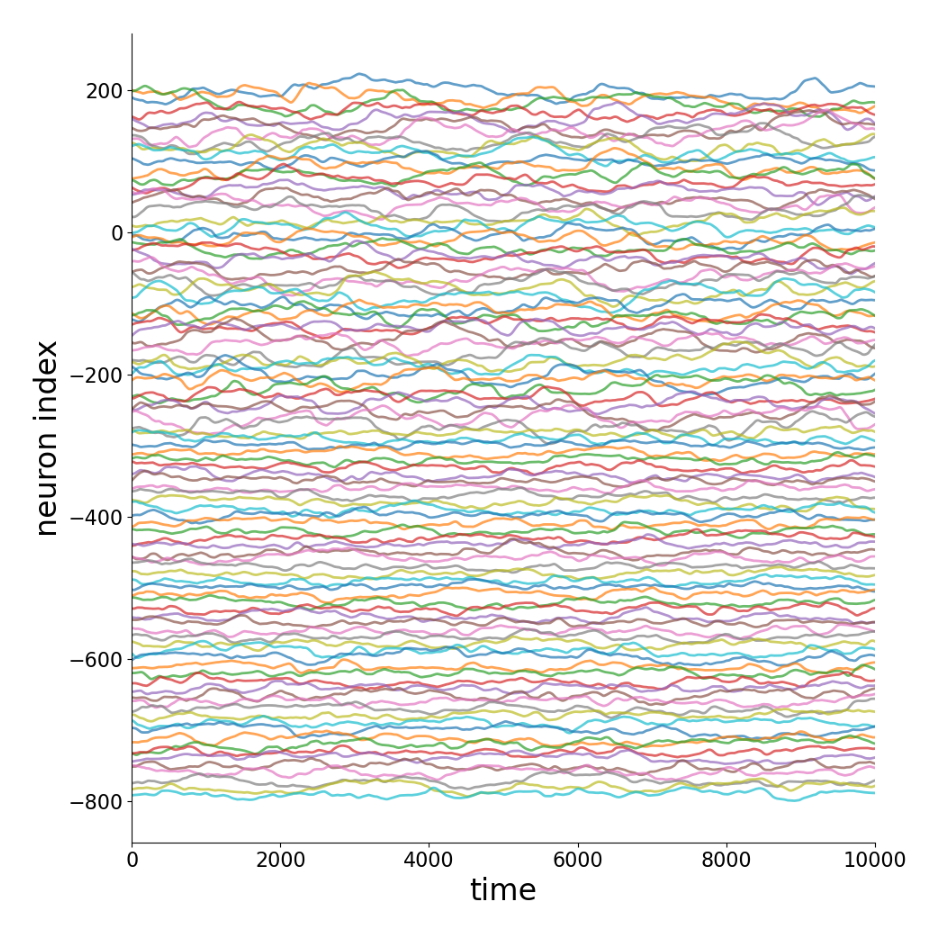
Generate synthetic neural activity data using the PDE_N2 model. This creates the training dataset with 1000 neurons over 100,000 time points.
Outputs:
Sample of 100 time series
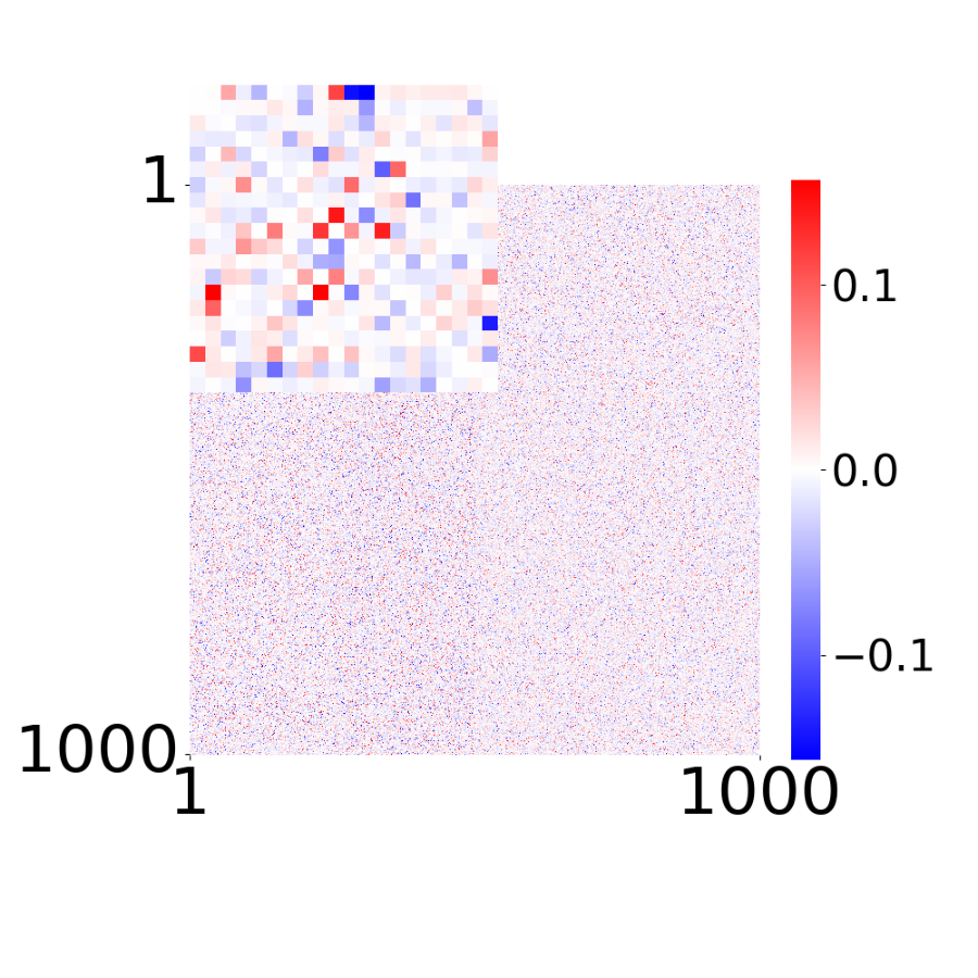
True connectivity matrix \(W_{ij}\)
Code
# STEP 1: GENERATE print ()print ("-" * 80 )print ("STEP 1: GENERATE - Simulating neural activity" )print ("-" * 80 )# Check if data already exists = f' { graphs_dir} /x_list_0.npy' if os.path.exists(data_file):print (f"data already exists at { graphs_dir} /" )print ("skipping simulation, regenerating figures..." )= device,= False ,= 0 ,= "color" ,= 1 ,= False ,= True ,= 2 ,= True ,else :print (f"simulating { config. simulation. n_neurons} neurons, { config. simulation. n_neuron_types} types" )print (f"generating { config. simulation. n_frames} time frames" )print (f"output: { graphs_dir} /" )print ()= device,= False ,= 0 ,= "color" ,= 1 ,= False ,= True ,= 2 ,
Step 2: Train GNN
Train the GNN to learn connectivity \(W\) and functions \(\phi^*/\psi^*\) (without latent embeddings). The GNN learns to predict \(dx/dt\) from the observed activity \(x\) .
The GNN optimizes the update rule (Equation 3 from the paper):
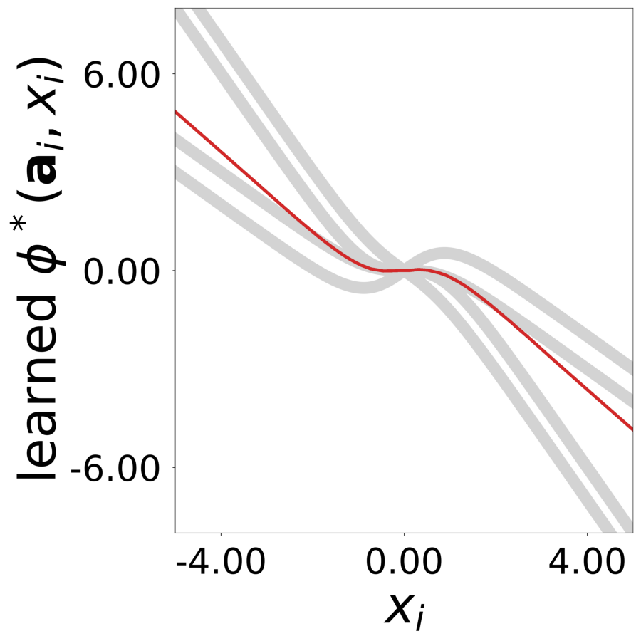
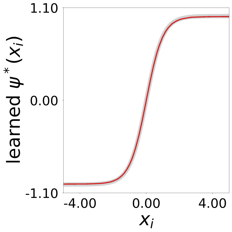
\[\hat{\dot{x}}_i = \phi^*(x_i) + \sum_j W_{ij} \psi^*(x_j)\]
where \(\phi^*\) and \(\psi^*\) are MLPs (ReLU, hidden dim=64, 3 layers) and \(W\) is the learnable connectivity matrix.
Code
# STEP 2: TRAIN print ()print ("-" * 80 )print ("STEP 2: TRAIN - Training GNN to learn W, phi, psi (no embeddings)" )print ("-" * 80 )# Check if trained model already exists (any .pt file in models folder) import glob= glob.glob(f' { log_dir} /models/*.pt' )if model_files:print (f"trained model already exists at { log_dir} /models/" )print ("skipping training (delete models folder to retrain)" )else :print (f"training for { config. training. n_epochs} epochs, { config. training. n_runs} run(s)" )print (f"learning: connectivity W, functions phi* and psi* (no embeddings)" )print (f"models: { log_dir} /models/" )print (f"training plots: { log_dir} /tmp_training" )print (f"tensorboard: tensorboard --logdir { log_dir} /" )print ()= config,= False ,= best_model,= 'color' ,= device
Step 3: GNN Evaluation
Figures matching Supplementary Figure 3 from the paper.
Figure panels:
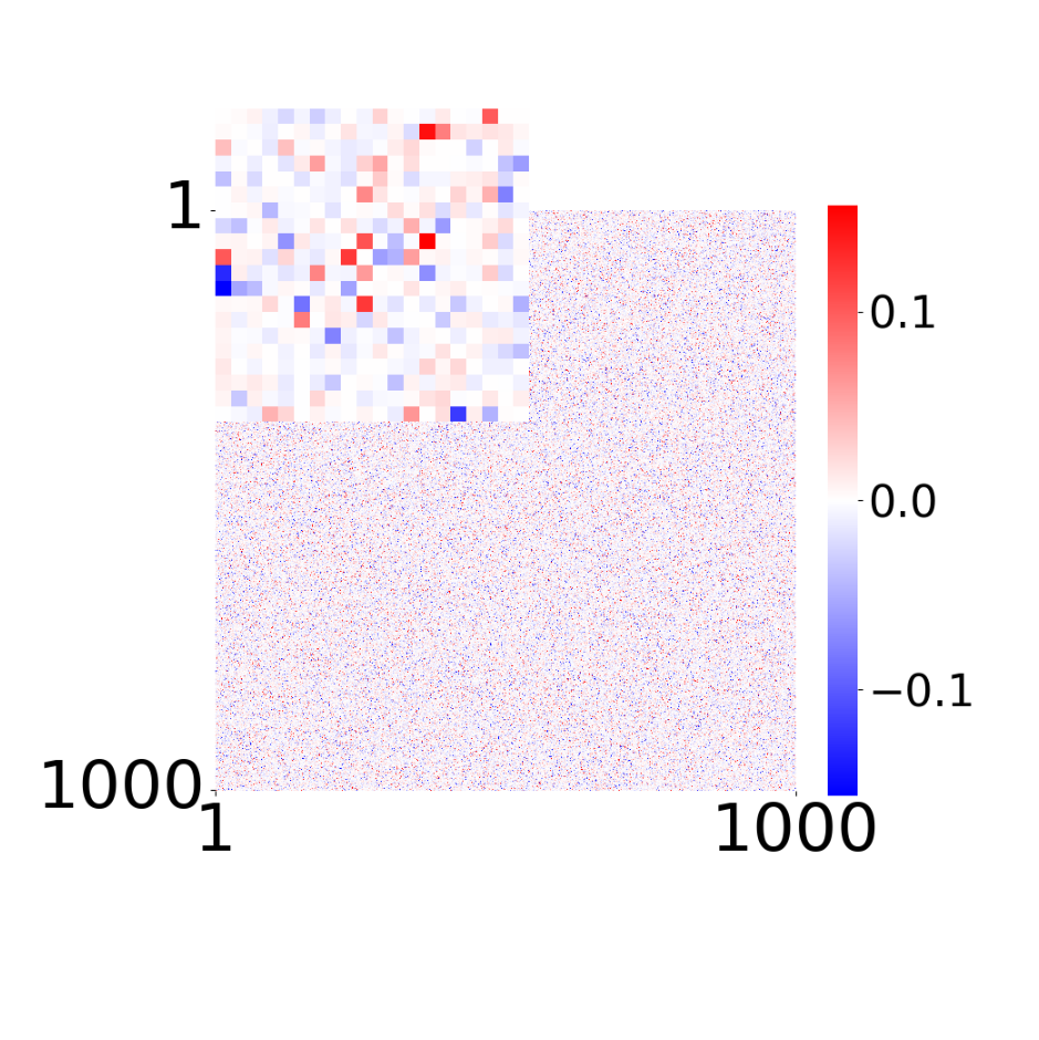
Supp. Fig 3d: Learned connectivity matrix
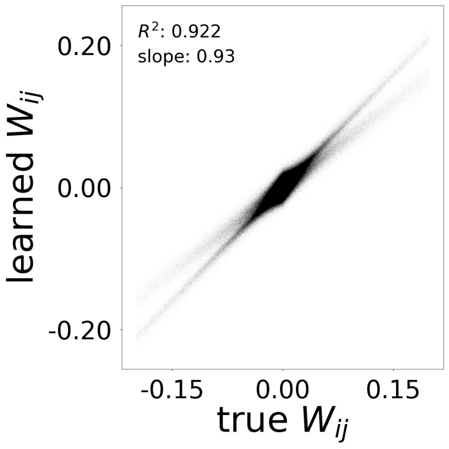
Supp. Fig 3e: Comparison of learned vs true connectivity
Supp. Fig 3g: Learned update functions \(\phi^*(x)\)
Supp. Fig 3h: Learned transfer function \(\psi^*(x)\)
Code
# STEP 3: GNN EVALUATION print ()print ("-" * 80 )print ("STEP 3: GNN EVALUATION - Generating Supplementary Figure 3 panels" )print ("-" * 80 )print (f"learned connectivity matrix" )print (f"W learned vs true (R^2, slope)" )print (f"update functions phi*(x)" )print (f"transfer function psi*(x)" )print (f"output: { log_dir} /results/" )print ()= './log/' + pre_folder + '/tmp_results/' = True )= config, config_file= config_file, epoch_list= ['best' ], style= 'color' , extended= 'plots' , device= device, apply_weight_correction= True , plot_eigen_analysis= False )
Step 4: Test Model
Test the trained GNN model. Evaluates prediction accuracy and performs rollout inference.
Code
# STEP 4: TEST print ()print ("-" * 80 )print ("STEP 4: TEST - Evaluating trained model" )print ("-" * 80 )print (f"testing prediction accuracy and rollout inference" )print (f"output: { log_dir} /results/" )print ()= 0.0 = config,= False ,= "color name continuous_slice" ,= False ,= 'best' ,= 0 ,= "" ,= False ,= 10 ,= 1000 ,= device,= 0 ,= None ,
Rollout Results
Display the rollout comparison figures showing: - Left panel: activity traces (ground truth gray, learned colored) - Right panel: scatter plot of true vs learned \(x_i\) with \(R^2\) and slope