Figure 2: baseline - 1000 neurons with 4 types

This script reproduces the panels of paper’s Figure 2 and other related supplementary panels (Supp. 1, 2, 5 and 6).

Simulation parameters:

• N_neurons: 1000
• N_types: 4 parameterized by \(\tau_i\)={0.5,1}, \(s_i\)={1,2} and \(g_i\)=10
• N_frames: 100,000
• Connectivity: 100% (dense)
• Connectivity weights: random, Cauchy distribution
• Noise: none
• External inputs: none

The simulation follows a simplified Equation 2 from the paper:

\[\frac{dx_i}{dt} = -\frac{x_i}{\tau_i} + s_i \cdot \tanh(x_i) + g_i \cdot \sum_j W_{ij} \cdot \tanh(x_j)\]

Configuration and Setup

print()
print("=" * 80)
print("Figure 2: 1000 neurons, 4 types, dense connectivity")
print("=" * 80)

device = []
best_model = ''
config_file_ = 'signal_fig_2'

print()
config_root = "./config"
config_file, pre_folder = add_pre_folder(config_file_)

# load config
config = NeuralGraphConfig.from_yaml(f"{config_root}/{config_file}.yaml")
config.config_file = config_file
config.dataset = config_file

if device == []:
    device = set_device(config.training.device)

log_dir = f'./log/{config_file}'
graphs_dir = f'./graphs_data/{config_file}'

Step 1: Generate Data

Generate synthetic neural activity data using the PDE_N2 model (src/neural-gnn/generators). This creates the training dataset with 1000 neurons of 4 different types over 100,000 time points.

Outputs:

• Figure 2b: Sample of 100 time series
• Figure 2c: True connectivity matrix \(W_{ij}\)

# STEP 1: GENERATE
print()
print("-" * 80)
print("STEP 1: GENERATE - Simulating neural activity (Fig 2a-c)")
print("-" * 80)

# Check if data already exists
data_file = f'{graphs_dir}/x_list_0.npy'
if os.path.exists(data_file):
    print(f"data already exists at {graphs_dir}/")
    print("skipping simulation, regenerating figures...")
    data_generate(
        config,
        device=device,
        visualize=False,
        run_vizualized=0,
        style="color",
        alpha=1,
        erase=False,
        bSave=True,
        step=2,
        regenerate_plots_only=True,
    )
else:
    print(f"simulating {config.simulation.n_neurons} neurons, {config.simulation.n_neuron_types} types")
    print(f"generating {config.simulation.n_frames} time frames")
    print(f"output: {graphs_dir}/")
    print()
    data_generate(
        config,
        device=device,
        visualize=False,
        run_vizualized=0,
        style="color",
        alpha=1,
        erase=False,
        bSave=True,
        step=2,
    )

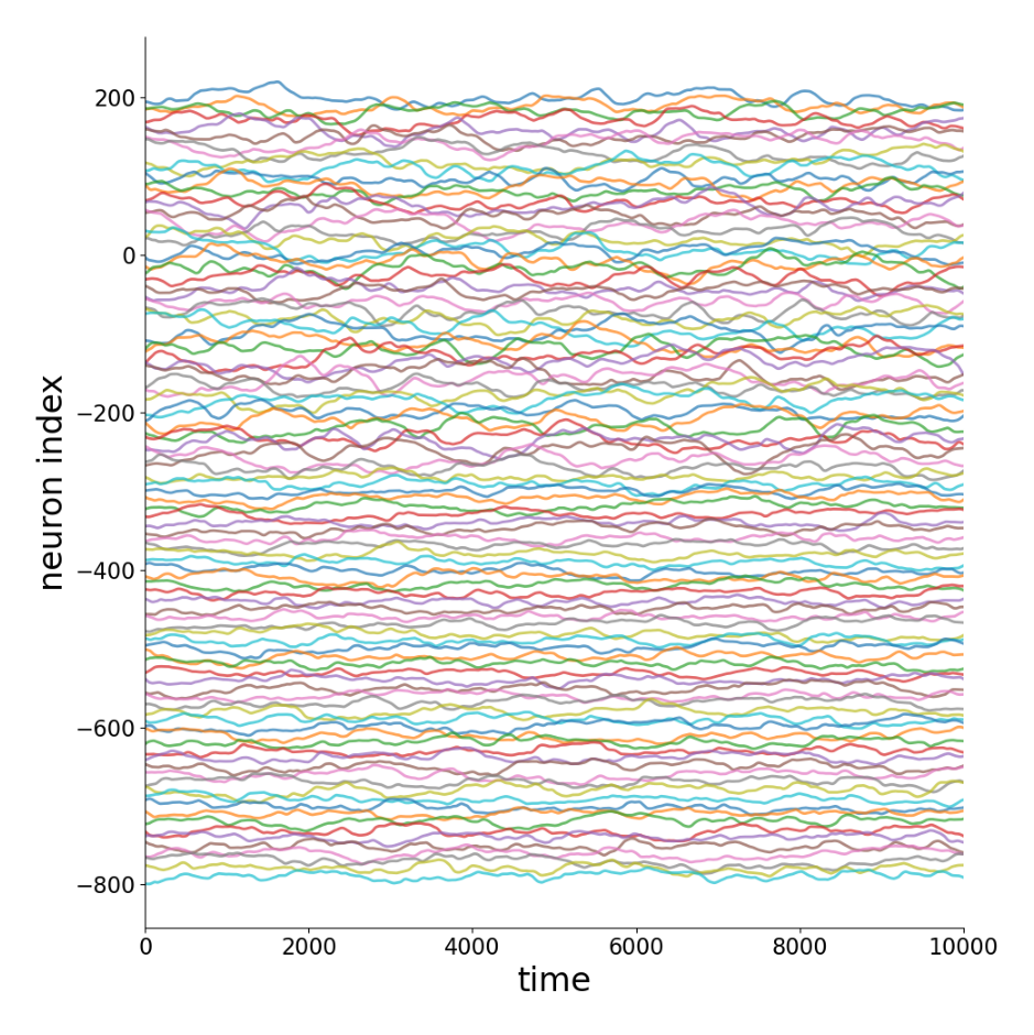
Fig 2b: Sample of 100 time series taken from the activity data.

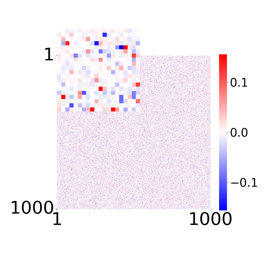
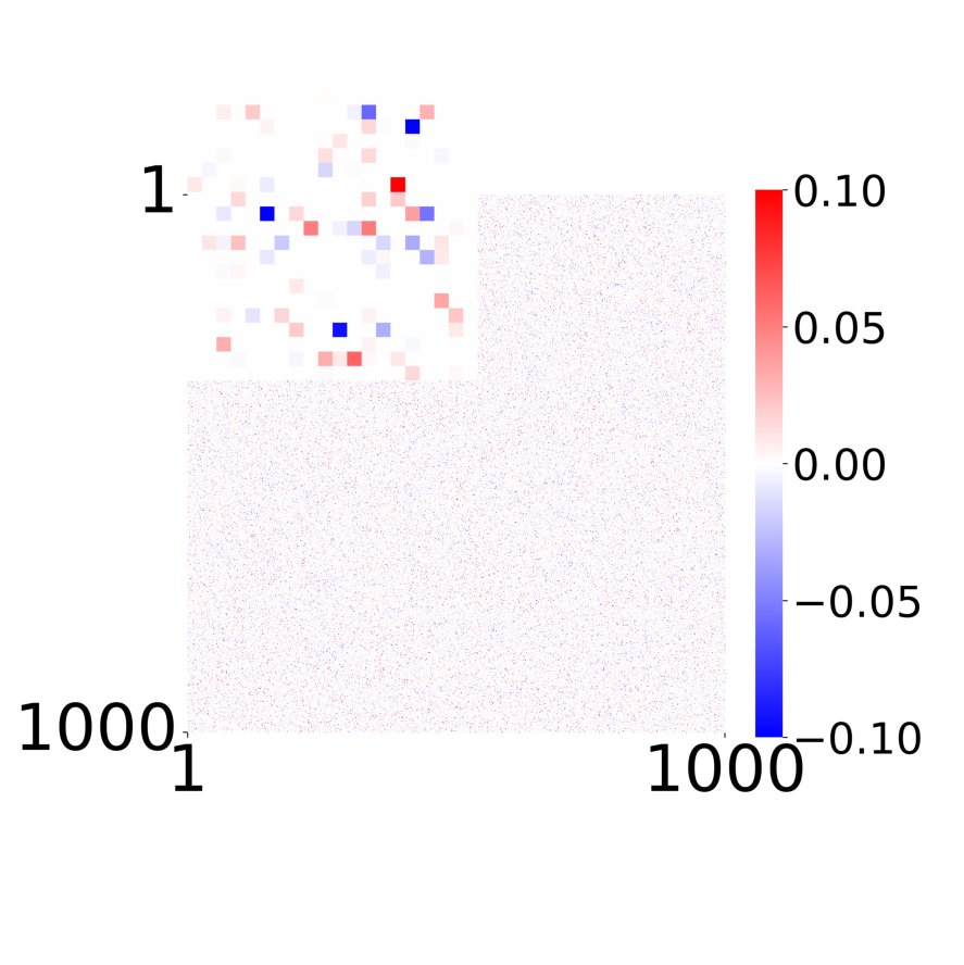
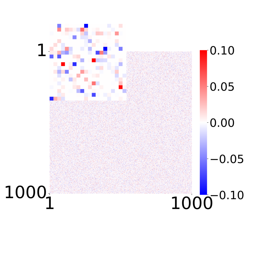
Fig 2c: True connectivity \(W_{ij}\). The inset shows 20×20 weights.

Step 2: Train GNN

Train the GNN to learn connectivity \(W\), latent embeddings \(\mathbf{a}_i\), and functions \(\phi^*, \psi^*\) with the SignalPropagation model (‘src/neural-gnn/models’). The GNN learns to predict \(dx_i/dt\) from the observed activity \(x_i\).

The GNN optimizes the update rule (Equation 3 from the paper):

\[\hat{\dot{x}}_i = \phi^*(\mathbf{a}_i, x_i) + \sum_j W_{ij} \psi^*(x_j)\]

where \(\phi^*\) and \(\psi^*\) are MLPs (ReLU, hidden dim=64, 3 layers). \(\mathbf{a}_i\) is a learnable 2D latent vector per neuron, and \(W\) is the learnable connectivity matrix.

# STEP 2: TRAIN
print()
print("-" * 80)
print("STEP 2: TRAIN - Training GNN to learn W, embeddings, phi, psi")
print("-" * 80)

# Check if trained model already exists (any .pt file in models folder)
import glob
model_files = glob.glob(f'{log_dir}/models/*.pt')
if model_files:
    print(f"trained model already exists at {log_dir}/models/")
    print("skipping training (delete models folder to retrain)")
else:
    print(f"training for {config.training.n_epochs} epochs, {config.training.n_runs} run(s)")
    print(f"learning: connectivity W, latent vectors a_i, functions phi* and psi*")
    print(f"models: {log_dir}/models/")
    print(f"training plots: {log_dir}/tmp_training")
    print(f"tensorboard: tensorboard --logdir {log_dir}/")
    print()
    data_train(
        config=config,
        erase=False,
        best_model=best_model,
        style='color',
        device=device
    )

Step 3: GNN Evaluation

Figures matching Figure 2, and supplementary Fig 1, 2, 5, and 6 from the paper.

Figure panels:

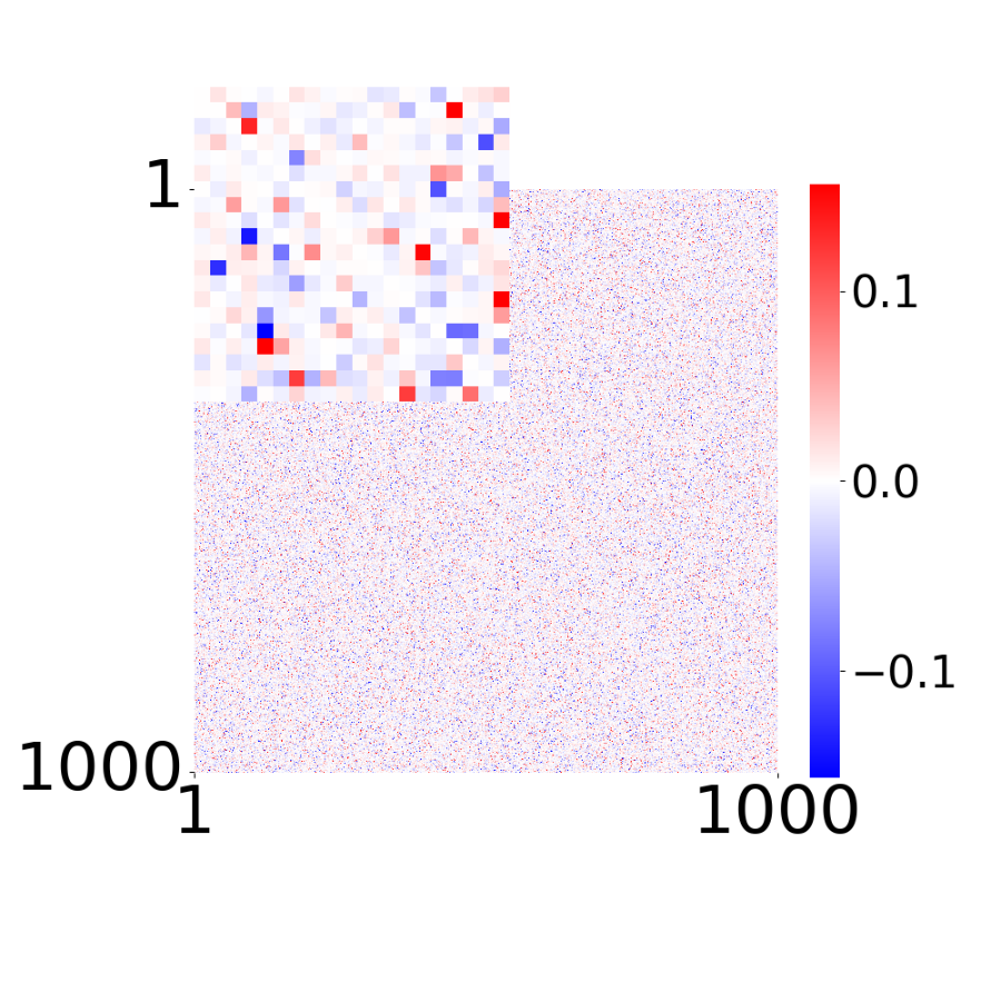
• Fig 2d: Learned connectivity matrix
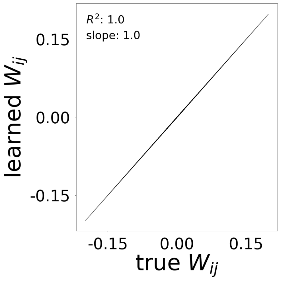
• Fig 2e: Comparison of learned vs true connectivity
• Fig 2f: Learned latent vectors \(\mathbf{a}_i\)
• Fig 2g: Learned update functions \(\phi^*(\mathbf{a}_i, x)\)
• Fig 2h: Learned transfer function \(\psi^*(x)\)

# STEP 3: GNN EVALUATION
print()
print("-" * 80)
print("STEP 3: GNN EVALUATION - Generating Figure 2 panels (d-h)")
print("-" * 80)
print(f"Fig 2d: Learned connectivity matrix")
print(f"Fig 2e: W learned vs true (R^2, slope)")
print(f"Fig 2f: Latent vectors a_i (4 clusters)")
print(f"Fig 2g: Update functions phi*(a_i, x)")
print(f"Fig 2h: Transfer function psi*(x)")
print(f"output: {log_dir}/results/")
print()
folder_name = './log/' + pre_folder + '/tmp_results/'
os.makedirs(folder_name, exist_ok=True)
data_plot(config=config, config_file=config_file, epoch_list=['best'], style='color', extended='plots', device=device, apply_weight_correction=True, plot_eigen_analysis=False)

Figures 2d-2h: GNN Evaluation Results

Fig 2d: Learned connectivity.

Fig 2e: Comparison of learned and true connectivity (given \(g_i\)=10).

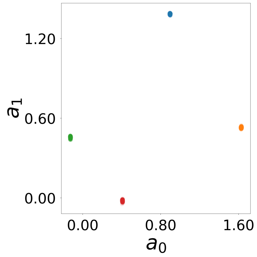
Fig 2f: Learned latent vectors \(a_i\) of all neurons.

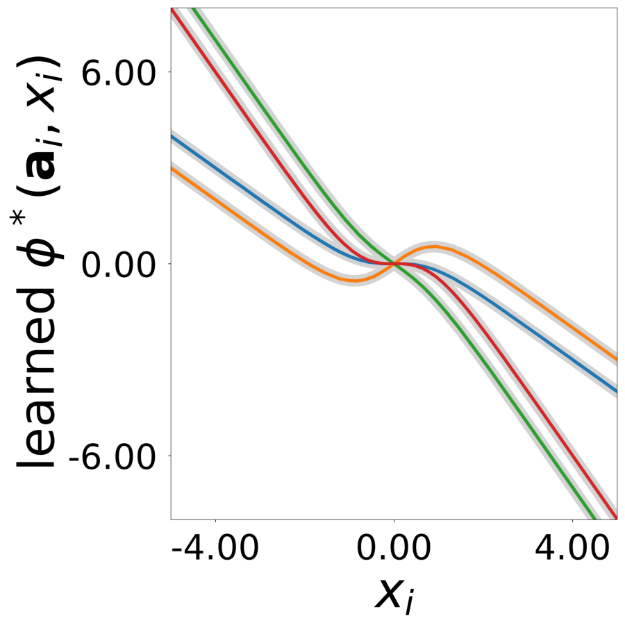
Fig 2g: Learned update functions \(\phi^*(a_i, x)\). The plot shows 1000 overlaid curves, one for each vector \(a_i\). Colors indicate true neuron types. True functions are overlaid in light gray.

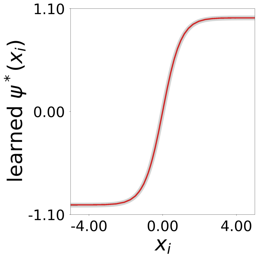
Fig 2h: Learned transfer function \(\psi^*(x)\), normalized to a maximum value of 1. True function is overlaid in light gray.

Step 4: GNN Training Visualization

Generate training progression figures showing how the GNN learns across epochs.

Visualizations:

• Row a: Latent embeddings \(\mathbf{a}_i\) evolution
• Row b: Update functions \(\phi^*(\mathbf{a}_i, x)\)
• Row c: Transfer function \(\psi^*(x)\)
• Row d: Connectivity matrix \(W\)
• Row e: \(W\) learned vs true scatter plot

# STEP 4: GNN TRAINING VISUALIZATION
print()
print("-" * 80)
print("STEP 4: GNN TRAINING - Generating training progression figures")
print("-" * 80)
print(f"generating plots for all training epochs")
print(f"output: {log_dir}/results/all/")
print()
data_plot(config=config, config_file=config_file, epoch_list=['all'], style='color', extended='plots', device=device, apply_weight_correction=True, plot_eigen_analysis=False)

# Create montage from individual epoch plots
print()
print("creating training montage (8 columns x 5 rows)...")
create_training_montage(config=config, n_cols=8)

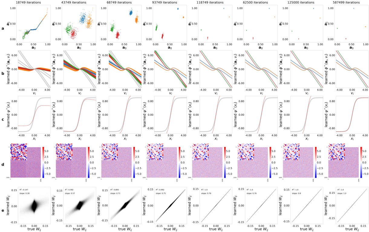
Supplementary Figure 1: Results plotted over 20 epochs. (a) Learned latent vectors \(a_i\). (b) Learned update functions \(\phi^*(a_i, x)\). (c) Learned transfer function \(\psi^*(x)\), normalized to max=1. (d) Learned connectivity \(W_{ij}\). (e) Comparison of learned and true connectivity. Colors indicate true neuron types.

Step 5: Test Model

Test the trained GNN model. Evaluates prediction accuracy and performs rollout inference.

# STEP 5: TEST
print()
print("-" * 80)
print("STEP 5: TEST - Evaluating trained model")
print("-" * 80)
print(f"testing prediction accuracy and rollout inference")
print(f"output: {log_dir}/results/")
print()
config.simulation.noise_model_level = 0.0

data_test(
    config=config,
    visualize=False,
    style="color name continuous_slice",
    verbose=False,
    best_model='best',
    run=0,
    test_mode="",
    sample_embedding=False,
    step=10,
    n_rollout_frames=1000,
    device=device,
    particle_of_interest=0,
    new_params=None,
)

Rollout Results

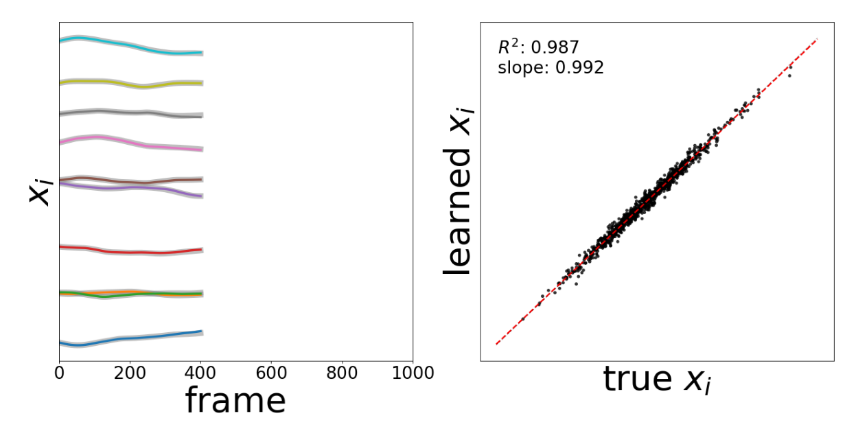
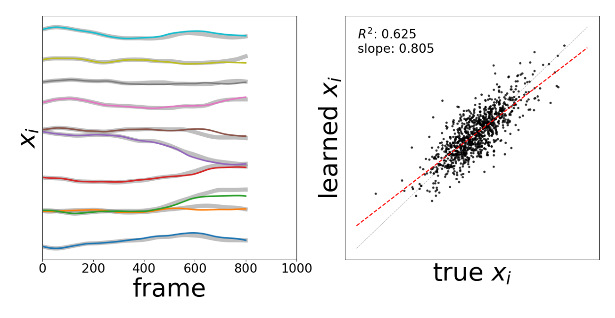
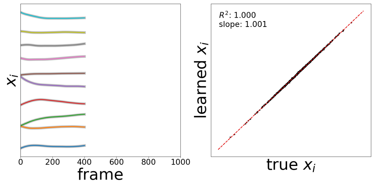
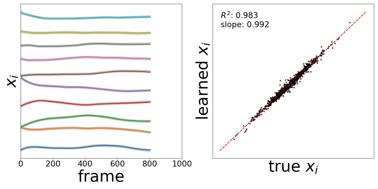
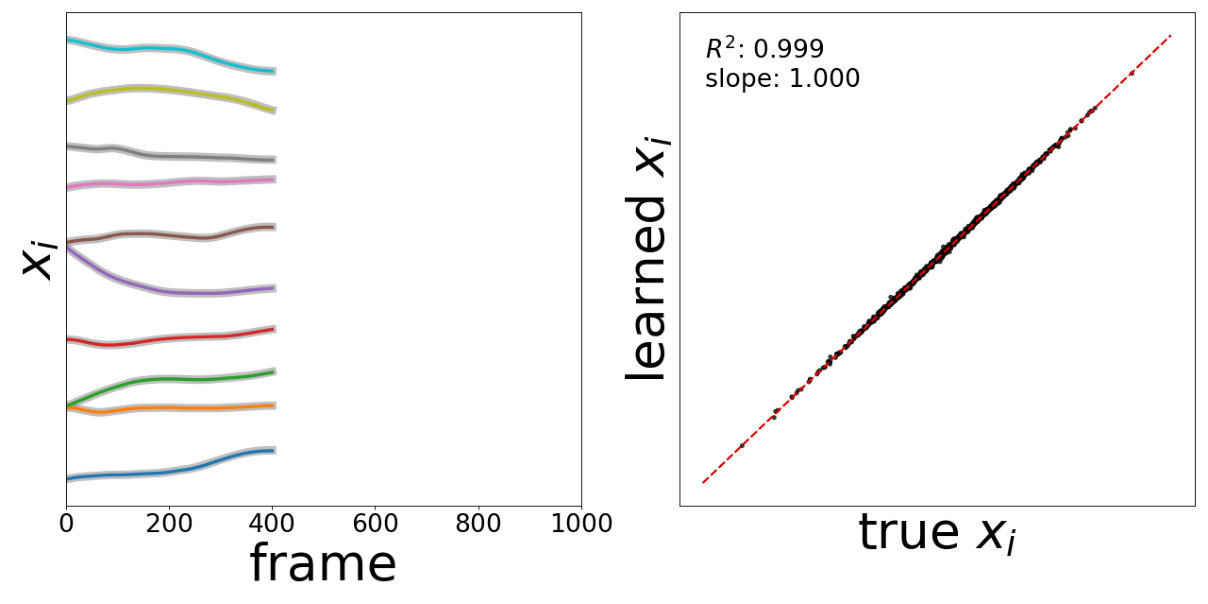
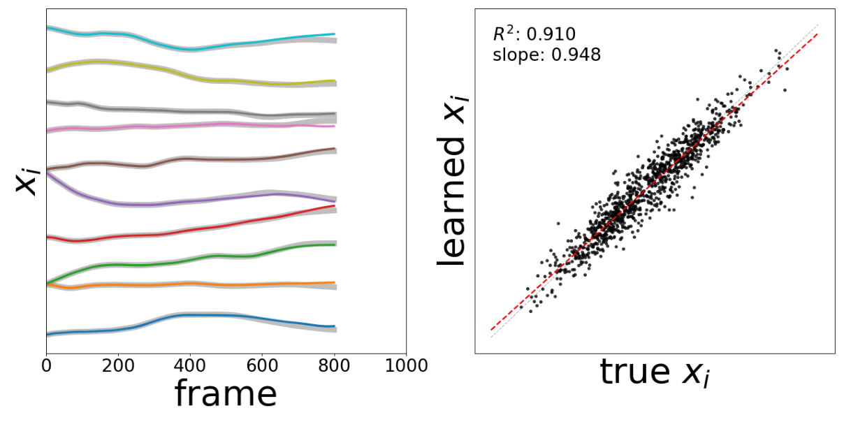
• Left panel: activity traces (ground truth gray, learned colored)
• Right panel: scatter plot of true vs learned \(x_i\) with \(R^2\) and slope

Rollout comparison up to time-point 400.

Rollout comparison up to time-point 800.

Step 6: Supplementary Figure 5 - Generalization Test

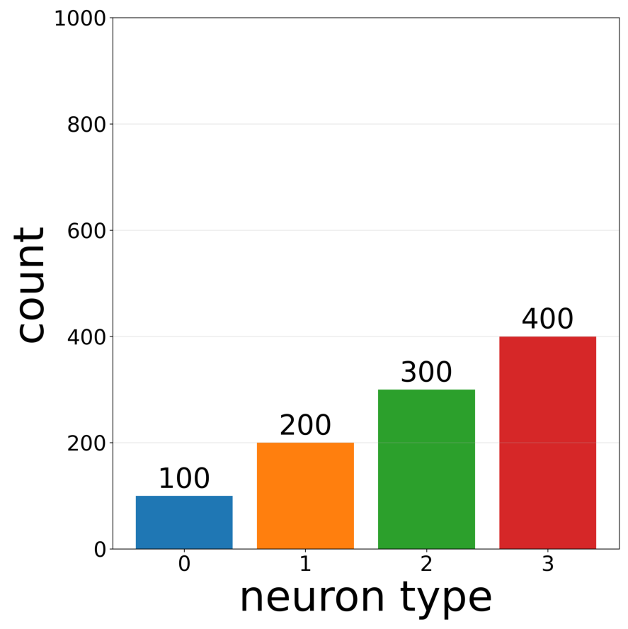
Test the trained GNN with modified network structure. Modified neuron type proportions (10%, 20%, 30%, 40% instead of 25% each) and modified sparse connectivity (~25% sparsity, 243,831 weights instead of 10^6).

Outputs:

• Panel b: Modified neuron type proportions histogram
• Panel d: Modified sparse connectivity matrix
• Panels e,f: Rollout at 400 time-points
• Panels g,h: Rollout at 800 time-points

# STEP 6: SUPPLEMENTARY FIGURE 5 - GENERALIZATION TEST
print()
print("-" * 80)
print("STEP 6: SUPPLEMENTARY FIGURE 5 - Generalization test with modified network")
print("-" * 80)
print("modified neuron type proportions: 10%, 20%, 30%, 40%")
print("modified connectivity: ~25% sparsity (243,831 weights)")
print()

# new_params: [connectivity_filling_factor, type0_pct, type1_pct, type2_pct, type3_pct]
new_params_supp5 = [0.25, 10, 20, 30, 40]

data_test(
    config=config,
    visualize=True,
    style="color",
    verbose=False,
    best_model='best',
    run=0,
    test_mode="",
    sample_embedding=False,
    step=10,
    n_rollout_frames=1000,
    device=device,
    particle_of_interest=0,
    new_params=new_params_supp5,
)

Supplementary Figure 5 Panels

Panel b: Modified neuron type proportions (10%, 20%, 30%, 40%).

Panel d: Modified sparse connectivity matrix (~25% sparsity, 243,831 weights).

Panels e,f: Rollout up to 400 time-points.

Panels g,h: Rollout up to 800 time-points.

Supplementary Figure 6 - Generalization Test

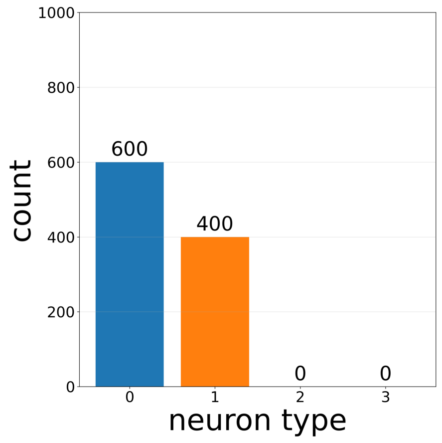
Test the trained GNN with network modifications. Modified neuron type proportions: 60%, 40%, 0%, 0% (types 2 and 3 eliminated) and modified sparse connectivity: ~50% sparsity (487,401 weights instead of 10^6).

Outputs:

• Panel b: Modified neuron type proportions histogram
• Panel d: Modified sparse connectivity matrix
• Panels e,f: Rollout at 400 time-points
• Panels g,h: Rollout at 800 time-points

# SUPPLEMENTARY FIGURE 6 - GENERALIZATION TEST
print()
print("-" * 80)
print("SUPPLEMENTARY FIGURE 6 - Generalization test with extreme network modification")
print("-" * 80)
print("modified neuron type proportions: 60%, 40%, 0%, 0% (types 2,3 eliminated)")
print("modified connectivity: ~50% sparsity (487,401 weights)")
print()

# new_params: [connectivity_filling_factor, type0_pct, type1_pct, type2_pct, type3_pct]
# 50% sparsity = 0.5 filling factor -> ~500,000 weights
new_params_supp6 = [0.5, 60, 40, 0, 0]

data_test(
    config=config,
    visualize=True,
    style="color",
    verbose=False,
    best_model='best',
    run=0,
    test_mode="",
    sample_embedding=False,
    step=10,
    n_rollout_frames=1000,
    device=device,
    particle_of_interest=0,
    new_params=new_params_supp6,
)

Supplementary Figure 6 Panels

Panel b: Modified neuron type proportions (60%, 40%, types 2,3 eliminated).

Panel d: Modified sparse connectivity matrix (~50% sparsity, 487,401 weights).

Panels e,f: Rollout up to 400 time-points.

Panels g,h: Rollout up to 800 time-points.